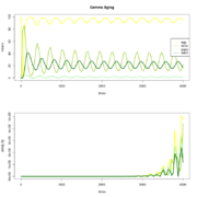

Fig 1 Code b=5, ue= 0, ul = 0.001, up = 0, ua = 0.01, ae = .13*k, al = .01*k, ap = .15*k, cle = .2, cap = .1, cae = 5, V=volume


Fig 2 b=5, ue= 0, ul = 0.001, up = 0, ua = .001, ae = .1*k, al = .01*k, ap = .1*k, cle = 1, cap = .4, cae = 1, V=volume
### System Size Expansion
Analytic calculation captures the noise propagation through the age structure correctly. This can lead to much larger estimates of the impact of demographic stochastically than previously believed.
This covariance mechanism requires coupling through the nonlinear terms, otherwise it can simply cancel out. The asymmetric, nonlinear term such as in the generalized crowley model seems to be the simplest way to produce a large demographic noise effect:

Earlier descriptions have failed to include the connections in the noise structure, i.e. from Dennis et al 2001 “that the noise variables are uncorrelated with each other within a time unit (off-diagonal elements of the matrix are zero).”
Two interesting side-questions have emerged – the influence of the two-step vs one-step transitions and the connections of multiple stages.
### Status of Noise in LPA Model
- Macroscopic dynamics

- A noisy larval population with stable adult population could be driven in the LPA model by weak damping in the larval class  relative to a strong covariance term amplifying fluctuations from another class,
  . As larval dynamics are connected only to egg dynamics and only through a_e, this makes the oscillations relatively small.
- The stable adult noise can be driven by strong damping or weak coupling 
Comparison to Dennis et al model
which assumes

Which underestimates the noise twice over, with no covariance and a noise based on a pure birth process (difference instead of sum of rates).
Continuing Beetles Research
- Sustained oscillations seem to be yielding divergent noise dynamics. Fig 1.
- Identical model in a different parameter regime, noise is essentially Poisson, with variances matching means within each stage, and no suggestion of the instability seen in the oscillating case. Fig 2.
- Extensions (two-step, phases) and break-downs of the approximation (see/discuss with Michael Samoilov and Adam Arkin)
Misc —-
embed any webpage in an oww page:
<html><iframe height="500px" width="1000px" src="https://two.ucdavis.edu/~cboettig"></iframe></html>