Trying to find a better way to summarize outputs of simulations,
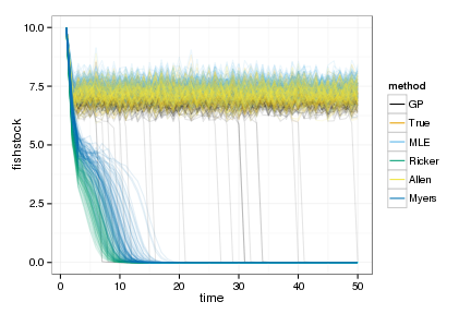
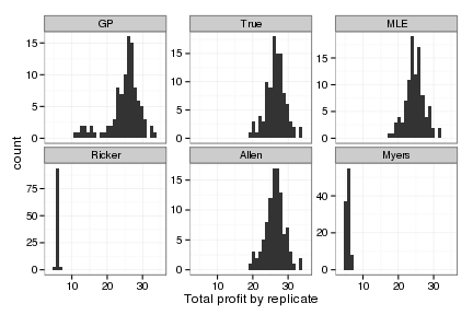
Heavy over-plotting makes the simulation trajectories themselves hard to read, even with transparent curves. Instead, we can plot the cumulative profit (technically should be discounted first):
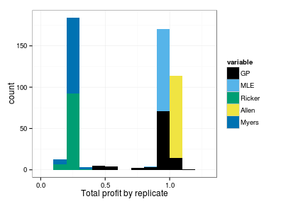
We can normalize these profits as a fraction of the theoretical optimum (true), providing a comparison that is less dependent on model parameters.

We can then attempt to plot these on a single plot, either as stacked histograms:
or stacked density plots:
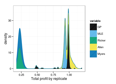
Even after (or because of) some tuning of binwidth I’m not sure I’m happy. Will probably go with the histogram. The density plot fails when distribution is purely a delta function, giving a uniform distribution instead (and is thus maximally wrong); this can be avoided by adding a small jitter.
- Code: see complete code nonparametric-bayes/fc6365
## @knitr Figure3
ggplot(sims_data) +
  geom_line(aes(time, fishstock, group=interaction(reps,method), color=method), alpha=.1) +
    scale_colour_manual(values=colorkey, guide = guide_legend(override.aes = list(alpha = 1)))


## @knitr profits
Profit <- sims_data[, sum(profit), by=c("reps", "method")]
tmp <- dcast(Profit, reps ~ method)
#tmp$Allen <- tmp[,"Allen"] + rnorm(dim(tmp)[1], 0, 1) # jitter for plotting
tmp <- tmp / tmp[,"True"]
tmp <- melt(tmp[2:dim(tmp)[2]])
actual_over_optimal <-subset(tmp, variable != "True")


## @knitr Figure4
ggplot(actual_over_optimal, aes(value)) + geom_histogram(aes(fill=variable)) +
  facet_wrap(~variable, scales = "free_y")  + guides(legend.position = "none") +
  xlab("Total profit by replicate") + scale_fill_manual(values=colorkey)

ggplot(actual_over_optimal, aes(value)) + geom_histogram(aes(fill=variable), binwidth=0.1) +
  xlab("Total profit by replicate")+ scale_fill_manual(values=colorkey)

ggplot(actual_over_optimal, aes(value, fill=variable, color=variable)) +
  stat_density(aes(y=..density..), position="stack", adjust=3, alpha=.9) +
  xlab("Total profit by replicate")+ scale_fill_manual(values=colorkey)+ scale_color_manual(values=colorkey)
Misc
Via Noam. Interesting
Richard interview
Exchange with Martin on links are citations Edit: it appears comments have been lost, but see discussion on the follow-up post, citations in scholarly markdown.
Wow, the scaling unit
emin LaTeX, CSS, etc. actually comes from the width of the characterM, dating back to printing-press era, when that character was used to define the spacing quadratone