After a few iterations I have a working minimal example (below). Hoping that ADMB is a bit more robust than vanilla optim out of R as I loop over data sets for the sensitivity analysis (#32). Does not seem to hold in simple example here, not sure why.
- These notes correspond to script 84a102/admb-example.md
Learning ADMB
Plotting and knitr options, (can generally be ignored)
Model and parameters
f <- function(x,h,p)  x * exp(p[1] * (1 - x / p[2]) * (x - p[3]) / p[2] )
p <- c(1, 10, 5)
K <- 10  # approx, a li'l' less
Xo <- 6 # approx, a li'l' less
Various parameters defining noise dynamics, grid, and policy costs.
sigma_g <- 0.1
z_g <- function() rlnorm(1,0, sigma_g)
x_grid <- seq(0, 1.5 * K, length=50)
Tobs <- 40
set.seed(123)
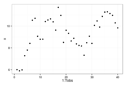
Sample Data
x <- numeric(Tobs)
x[1] <- Xo
for(t in 1:(Tobs-1))
  x[t+1] = z_g() * f(x[t], h=0, p=p)
qplot(1:Tobs, x)
Maximum Likelihood “by hand”
STABLIZE = 1e-10
n = length(x)
mloglik <- function(pars){
  r = pars[1]; k = pars[2]; c = pars[3]; s = pars[4];
  mu = (x+STABLIZE) * exp( r * (1 - x / (k+STABLIZE)) * (x - c) / (k + STABLIZE));
  mu = pmin(1e100, mu) # avoid infinite values
  f = 0.5 * n * log(2 * pi) + n * log(s + STABLIZE) + 0.5 * sum(x - mu + STABLIZE)^2/ (s + STABLIZE)^2;

  f
  }
Starting from the true values we mostly just shrink the noise parameter:
init <- c(p, sigma_g)
mloglik(init) #true minus loglik
[1] -35.72o <- optim(init, mloglik, method="L", lower=1e-5, upper=1e5)
o$value[1] -247.6o$par[1] 0.9967297 9.9813554 5.1742699 0.0008183While starting from arbitrary values we still find the optim.
init <- c(1,1,1,1)
init <- c(p, sigma_g)
mloglik(init) #true minus loglik
[1] -35.72o <- optim(init, mloglik, method="L", lower=1e-5, upper=1e5)
o$value[1] -247.6o$par[1] 0.9967297 9.9813554 5.1742699 0.0008183Okay, now lets try admb. We use R2admb which is just a convenient way to write our data and parameters into an admb file.
# install_github("R2admb", "bbolker", subdir="R2admb") # dev version
library(R2admb)
ADMB definition
We still need to define the model using ADMB notation in the procedure section. This is mostly like R or C++, with the exception of special functions like square in place of ^2, norm2 for the sum of squares, and elem_prod istead of * for the element-wise product of two arrays. The constant pi is given as M_PI, as typical of C/C++ libraries. Where these other functions are defined I’m not sure, but some useful guides to ADMB vector/matrix operations or an (undefined) list of keywords…
The equivalent model
model <-
paste("
PARAMETER_SECTION
  vector mu(1,n) // per capita mort prob

PROCEDURE_SECTION
  mu = log(x) + r * elem_prod((1 - x / k), (x - c) / k);
  f = 0.5 * n * log(2 * M_PI) + n * log(s) + 0.5 * norm2(x - exp(mu)) / square(s);
")
writeLines(model, "model.tpl")
Without explicit handling of the overflow errors, ADMB does not give us reliable estimates with arbitrary starting conditions
setup_admb("/var/admb")[1] "/var/admb"
df <- data.frame(x=x)
params <- list(r = 1, k = 1, c = 1, s = 1) ## starting parameters
bounds <- list(r = c(1e-10, 1e3), k=c(1e-10, 1e3), c=c(1e-10, 1e3), s = c(1e-5,1e3)) ## bounds
dat <- c(list(n = nrow(df)), df)
m1 <- do_admb("model",
              data = dat,
              params = params,
              bounds = bounds,
              run.opts = run.control(checkparam="write",
                                     checkdata="write", clean=FALSE))
m1
Model file: model_gen
Negative log-likelihood: 146.5
Coefficients:
r k c s
0.9992 1.0023 1.0004 9.4369 But does fine with good starting values. Hmm.. thought that was supposed to be the other way around…
params <- list(r = 1, k = 10, c = 5, s = .1) ## starting parameters

m1 <- do_admb("model",
              data = dat,
              params = params,
              bounds = bounds,
              run.opts = run.control(checkparam="write",
                                     checkdata="write"))
Warning: running command './model_gen > model_gen.out' had status 1m1Model file: model_gen
Negative log-likelihood: -423.8
Coefficients:
r k c s
2.025e-10 9.498e+00 1.051e+01 1.000e-05 Which finds a better optim (though substantailly overfit in reality)
Hans suggests adding an error term in the function definitions rather than in limiting the bounds or log transforming the variables:
The most common plase where this goes wrong is 1/0, log(0), sqrt(0), pow(0,1) etc. Your suggestion is OK, but usually I prefer to put in log(1e-10+my_expression), sqrt(1e-10+my_expression), pow(1e-10+my_expression,1)
Misc
Finished off posts regarding DOIs and digital archiving. A shorter version appears in my answer to opendata.stackexchange on blog archiving.
Interesting discussion on using PURL redirects with SHA hash to link to repositories. For instance, the commit matching our arXiv submission of the ews-review paper is found at cboettig/ews-review/33dfb58e24ceb5861dad7cf756cffe2c5d66a655. If the hash shown in the PURL doesn’t match the one at the repository then we know something has gone wrong, since it is impossible to change the contents without changing the hash. This gives us a version-stable identifier that can always be remapped to this commit, even if Github should disappear. Of course nothing guarentees that the PURL maintainer / package author does this updating, but in principle the system is more robust than simply linking to Github.
In other news, I should add some automatic link checking, #94 to the notebook.