Working from the quadratic model for the saddle node bifurcation rather than the linear (OU) model. Recall that the dynamics are:
\[dX = \left( r - (x-\theta)^2\right)dt + \beta \sqrt{X} dB_t \]
and the linear noise approximation gives a linear Fokker Planck equation such that the probability distribution is Gaussian with moments ((corrected from yesterday to scale noise, basically as pure-birth Poisson process))
\[\frac{d \hat{x}}{dt} &= r - (\hat{x}-\theta)^2 \] \[ \frac{d \sigma^2}{dt} &= -2 (\hat x - \theta )\sigma^2 + \beta \left(r - (\hat{x}-\theta)^2 \right) \]
So we can evaluate the probability density of being at $ x_t$ at time t given that we started at x_0 at time 0 by integrating the above equations (numerically, in this case, as we lack a closed form solution for the above).
Being able to calculate this probability we can easily calculate likelihood of the timeseries under the model. We code this in R (likelihood_bifur_models.R) and write a quick example script (also in repo as bifur_likelihood_ex.R):
pars = c(r=10, theta=3, beta=1)
m <- init_sdemodel(pars =pars, Xo = 6.2, model="SN", N=200)
X <- simulate.SN(m)
# Set initial guess
m$pars <- c(r=11,theta=4,beta=1)
out <- update.SN(m, X, method="SANN")
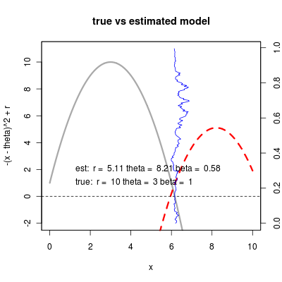
Exploring different fitting, seems to be a challenge. For instance, finds wrong optimum sometimes – perhaps due to a bug somewhere (see more examples in flickr stream): 
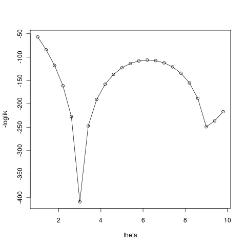
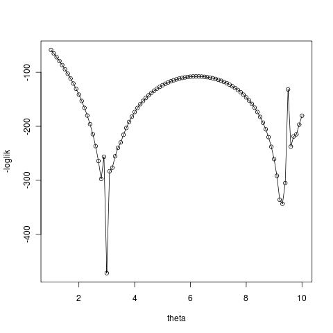
As likelihood surface (shown here for theta) appears challenging:

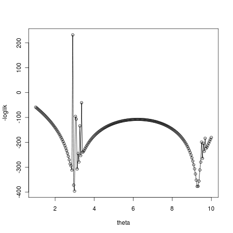
and numerical errors make it worse:


Never the less, the fit does okay when the initial condition for theta starts nearer the better well (right). See flickr library for more examples and git for code. Still not obvious why the unstable equilibrium is quite such a likelihood peak, but anyway…
Success of fits varies quite a bit, depending on data, initial guesses for parameters, etc. Note that for many of these the optimization fails to converge (more reasons discussed below).
[flickr-gallery mode=“tag” tags=“quadraticfitslides” tag_mode=“all”]
Improving automated recording in figures
Have added a git commit message to the reporting, so that flickr images are automatically tagged with a commit stamp referring to the script which produced them:
gitcom <- system('git commit -a -m "autocommit"', intern=TRUE)
# only first line of git commit commandline return will be printed in flickr discription
system(paste('flickr_upload --tag="stochpop bifurcation"', '--description="', gitcom, '"',  ' saddle_node_fit.png'))
system(paste('hpc-autotweets "', gitcom, ' done"'))
Would be nice to eventually make this a link. Also still good to print the most interesting parameters directly on the figure (or in the description if that isn’t appropriate) so that one doesn’t have to reference the code. Wonder if I can dump a larger text output into a single continuous string for the description.