I have often observed (e.g. Boettiger & Hastings (2012) ) that if purely stochastic transitions out of a potential well happen, then they happen fast (dispite the fact that waiting time for them to happen is very long). Yesterday Marc mentioned an interesting proof of this from Don Ludwig, who was able to show that the waiting time to reach a large deviation in a time \(t\), given that it reaches it at all, is of the same order as the return time from the large deviation to the equilibrium, \(\log(L/\sigma)\). That’s an absolutely fascinating conclusion, indeed a bit stronger than even I had expected (the waiting time until an escape is observed rather different! – of order \(\exp(L^2/\sigma^2)\).
Don’s derivation is repeated in pages 302-311 Marc’s “Theoretical Biologist’s Toolbox,” rather delightfully too (e.g. the “Kumura Maneuver”, or sidenotes such as “it is also kind of fun to do a web search with key words ‘Dawson’s Integral’”). Lande (1985) provides a somewhat different derivation of the same result.
Return time
The return time calculation is straight forward. Consider our OU model
\[dX = - X dt + \sigma dB_t\]
We ask for the return time into a neighborhood \(\sigma\) of the origin, starting at \(X_0 = L\) distant from the origin. The deterministic solution
\[ \tfrac{dx}{dt} = - x \]
implies $x_t = L (1 - e^{-t}) $, so setting \(x_t = \sigma_t\) and solving for \(t\), we find that \(x_t\) is within \(\sigma\) of \(t\) in time \(\log{L} - \log{\sigma}\), or \(\log{L/\sigma}\), as claimed.
Waiting time
The time we must wait before any trajectory can reach a given boundary is a classic hitting-time problem for the OU process that can be solved in several ways. Any of these basically start from PDE that must be satisfied for the hitting time (e.g. see Crispin Gardner, Stochastic Methods) for the OU process at stationary state (\(T_t = 0\)),
\[ \tfrac{\sigma^2}{2} T_{xx} - x T_x = -1 \]
With the appropriate boundary conditions \(T(L) = T(-L) = 0\). A little integration (see Dynkin’s formula) shows this scales as \(\exp(L^2/\sigma^2)\) (Compare to the Brownian walk that doesn’t have to escape any pull, which escapes at rate \(L^2/\sigma^2\).
Exit time
Most trajectories will thus return many times to the origin (stable point) before finally escaping. But if we focus just on the part of the trajectory from some value near the origin, that eventually escapes without ever crossing the origin again,
\[u_t(x,t) dt = Pr\left(\textrm{exit from }(0; L]\textrm{in the interval } (t, t + dt) \textrm{without having crossed} 0 | X(0) = x\right)\]
We are interested in comparing the average time taken by trajectories exiting by time \(t\) relative to the probability of exiting at all (i.e. as \(t \to \infty\)),
\[ T_c(x) = \frac{\int^{\infty}_0 t u_t(x,t) dt }{\lim_{t \to \infty} u(x,t) }\]
From here we set up the classic hitting time solution for the OU for the time-dependent PDE,
\[u_t = \frac{\sigma^2}{2} u_{xx} = x u_x \]
and with initial condition \(u(x,t=0) = 0\), \(u(0,t) = 0\), and \(u(L, t) = 1\). A bit of effort and an approximation to Dawson’s integral for \(L \gg x\) leads Don to bound the mean time to exit,
\[T_c(x) < \frac{1}{\sigma} \log\left(\frac{L}{\sigma}\right)\]
as claimed.
Results from Marc’s other suggestion
Marc also suggested exploring this by directly comparing steps left and right. A related way to measure the relative number of steps in the positive direction relative to the negative direction is Kendall’s tau rank correlation coefficient, which also looks at the number of increases relative to the number of decreases.
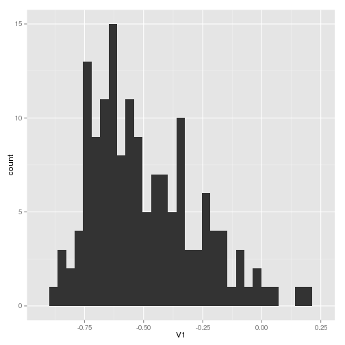
I’ve computed this statistic for my sample trajectories and plotted as a histogram here. The negative skew shows the tendancy to decrease (which is the direction of the deviation I selected – smaller population sizes)
I’ve also computed the ratio of steps up to steps down and histogrammed that: like the above, it shows more steps down than up, though not as dramatic as I might think by any means. Have to think about the role of the step size between observations in formulating this perhaps.

For the sake of completeness:
I may try and add a demonstration of Ludwig’s result above when I get some more free time to fiddle; will just need to add some additional simulations of return trajectories.
References
- C. Boettiger, A. Hastings, (2012) Early Warning Signals And The Prosecutor’S Fallacy. Proceedings of The Royal Society B: Biological Sciences 279 4734-4739 10.1098/rspb.2012.2085
- R Lande, (1985) Expected time for random genetic drift of a population between stable phenotypic states. Proceedings of the National Academy of Sciences https://www.pnas.org/content/82/22/7641.abstract