Summary Paragraph
- Critical transitions exist (Holling, 1973), (May, 1977),(Scheffer et. al. 2001)
- Warning signals exist (Scheffer et. al. 2009), (Drake & Griffen, 2010)
- Warning signals are summary statistics, critical slowing down (Wissel, 1984).
- Statement of general problem: double-edged sword – no quantification of the chance detection scheme will fail.
- We provide a way to do this
- We find existing methods lack sufficient power and have high false-alarm potential
- We provide a model-based solution using machinery of modern likelihood statistics
Background
- Define CSD, standard detection scheme. Figure 1.
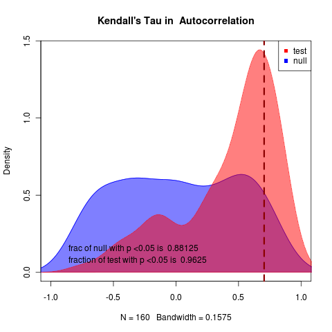
- What’s wrong with this approach: Figure 2
- We do not have a quantification of risk –> related to:
- We do not have a method designed for single replicates.
Being precise: expected value stationary process statistical independence
Consider an ensemble of data time series data which we represent as a matrix whose columns are replicates and rows are observations at each point in time. If they are produced by the same stationary process, then computing function f across the rows that returns a scalar value
Limits to Detection
We estimate probability of a missed event and false alarm. Even negative correlations can correspond to real events, while stable systems are quite likely to have strong signals.

To do this we need models.
Models for Critical Transitions
- General classes: Linearized transcritical, Linearized saddle node
- Models are: general, stochastic (can simulate), analytically tractable (can calc likelihood)
- Apply parametric bootstrap
Improving Power by Likelihood
Given that we’re comparing models there’s a full machinery to do this in a way that quantifies uncertainty. We follow Neyman-Pearson, Cox, McLachlan, Goldman, Huelsenbeck style (Compare Cox’s delta statistic for maximum likelihood estimates of models). Same basic Monte Carlo framework, but more powerful.
Avoid other bifurcation types:
i.e. Hastings & Wysham(Hastings & Wysham, 2010), or supercritical Hopf, see Sebastian’s examples(Schreiber, 2003)(Schreiber & Rudolf, 2008)), these would fail model adequacy, while summary-statistics approaches will not. (May need to outline this better with examples).
Conclusion
Serious application of warning signals must check for power.
We must quantify uncertainty.
Future is Bayesian approaches.
Methods options:
- put 200 words in main text under “Methods.” Or:
- put 300 words in “Methods Summary” at end of text (following figure legends).
- put 1000 words in “Additional Methods”.
You still need 300 word version as a “Methods Summary” for print.
“Additional” appears in online html only. This must repeat any critical info from the Summary (along with references). It cannot use figures or tables, but should have short bold headings. Cannot duplicate anything in the Supplement.
Option (B) is probably best, and just say “see supplement for details”. (As Drake 2010 does).
Appendices
Models
Parametric Bootstrap
Likelihood, AIC
Examples
MISC
Quantifying risk → realizing we often don’t have power to detect → improving power with likelihood approach.
But also mention issues like we address the single replicates problem, (also less vulnerable to applying in the case when the bifurcation is the wrong type, because models won’t fit well, but everything has a variance so you don’t realize you’re applying the wrong theory…)
Replacing prophesy with Science
risk – probability – chance
References
Holling C (1973). “Resilience And Stability of Ecological Systems.” Annual Review of Ecology And Systematics, 4. ISSN 0066-4162, https://dx.doi.org/10.1146/annurev.es.04.110173.000245.
May R (1977). “Thresholds And Breakpoints in Ecosystems With A Multiplicity of Stable States.” Nature, 269. ISSN 0028-0836, https://dx.doi.org/10.1038/269471a0.
Scheffer M, Carpenter S, Foley J, Folke C and Walker B (2001). “Unknown.” Nature, 413. ISSN 00280836, https://dx.doi.org/10.1038/35098000.
Scheffer M, Bascompte J, Brock W, Brovkin V, Carpenter S, Dakos V, Held H, van Nes E, Rietkerk M and Sugihara G (2009). “Early-Warning Signals For Critical Transitions.” Nature, 461. ISSN 0028-0836, https://dx.doi.org/10.1038/nature08227.
Drake J and Griffen B (2010). “Early Warning Signals of Extinction in Deteriorating Environments.” Nature, 467. ISSN 0028-0836, https://dx.doi.org/10.1038/nature09389.
Hastings A and Wysham D (2010). “Regime Shifts in Ecological Systems Can Occur With no Warning.” Ecology Letters, 13. ISSN 1461023X, https://dx.doi.org/10.1111/j.1461-0248.2010.01439.x.
Schreiber S and Rudolf V (2008). “Crossing Habitat Boundaries: Coupling Dynamics of Ecosystems Through Complex Life Cycles.” Ecology Letters, 11. https://dx.doi.org/10.1111/j.1461-0248.2008.01171.x.
- Sebastian J. Schreiber, (2003) Allee Effects, Extinctions, And Chaotic Transients in Simple Population Models. Theoretical Population Biology 64 10.1016/S0040-5809(03)00072-8
C. Wissel, (1984) A Universal Law of The Characteristic Return Time Near Thresholds. Oecologia 65 10.1007/BF00384470