Likelihood Calculation

Direct Calculation of the Joint Probability

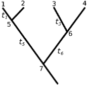
Fig 1 Sample tree

This is the approach implemented in the wrightscape project matrix_method.c. Consider an example phylogenetic tree (Fig 1) over which a stochastic process describes the evolution of trait x, defined by the transition probability rate w. Then the joint probability for a set of observed traits under this process can be written:

\begin{align} P(x_1, x_2, x_3, x_4) =& \int d x_7 \Biggl[ \left[ \int d x_5 w(x_7, x_5, t_5) w(x_5, x_1, t_1) w(x_5, x_2, t_1) \right] \\ & \times \left[ \int d x_6 w(x_7, x_6, t_6) w(x_6, x_3, t_3) w(x_6, x_4, t_3) \right] P(x_7) \Biggr] \end{align}

The transition density from any state to any state can be represented as a matrix over the domain of the integral. So at each node, we have a transition probability of entering any state that node can assume from any state from which its ancestor could assume. Though we have an analytical expression for this probability, we must evaluate it n² times for each matrix, then perform the matrix multiplications that are the equivalent discretization of the integral formulation above. If the tips are known they are represented instead by a single column of that matrix – i.e. transitions from any state to the known tip state. So:
Taking the element-wise product (denoted *) of the tip vectors times the matrix (chalkboard boldface) of the internal node prunes that node down to a single vector, and this can be recursed:

\int d x_5 w(x_7, x_5, t_5) w(x_5, x_1, t_1) w(x_5, x_2, t_1) \approx \mathbb{W}_5 (\vec W_1 * \vec W_2) \to \vec W_5

See implementation in the code, matrix_method.c.
While the discretization is substantially faster than the numerical integration, since it reduces the problem to a series of matrix products (note that given the root note and all tip nodes, then this produces a joint probability as a single scalar. Unknown tips results in a tensor, indicating the dimensionality of the full data space).
Most of the time is spent computing the elements of the matrices at each node, see Yesterday’s entry, which reduces performance to substantially below that of the linear likelihood schemes compared in that model. The advantage of this approach is that the W matrices can be computed in principle for any process, and once computed the actual calculation of the joint probability (the recursive integrals) occurs very fast, even for reasonably large grids. (No matrix inversion, just products!) It is rather the calculation of each element of the matrix separately that is both the rate limiting step and leads to poor (quadratic) scaling of compute time with increasing grid resolution. This leads us to consider some other approaches:

### Given a painting

Given a painting we can determine the likelihood of this regimes model (mixtures of OUs) with given parameter values (i.e. using the OUCH framework). For instance, if we assume as OUCH does, that for OU processes, *d**X* = α(θ − X)*d**t* + σ*d**B*_t,

sigma and alpha are global parameters but there can be different values of theta under regimes, then the joint probability is still multivariate normal, so its likelihood is given by

f_X(x) = \frac{1}{ (2\pi)^{k/2}|\Sigma|^{1/2} } \exp\!\Big( {-\tfrac{1}{2}}(x-\mu)’\Sigma^{-1}(x-\mu) \Big),

The addition of regimes with different thetas alters the calculation of the means, which can still be done using the solution to the expectation of the OU process. For instance, a tip that has spent time t₁ in regime 1 followed by time t₂ in regime 2 has expectation:

E(X) = (X_0 e^{-\alpha_1 t_1} + \theta_1) e^{\alpha_2 t_2} + \theta_2

and so forth. If we assume alpha and sigma are the same for all processes than the variance calculation is unaltered. We could also generalize this to allow regimes to change at points other than nodes, though in practice this may be unimportant. For varying alpha and sigma, we would need to modify the variance calculation (will hopefully write down soon). So all this is well implemented given the tree, but our desire is to avoid having to specify a painting.

Speed in this method depends largely on the ability to calculate distances between nodes on a tree. While many common implementations of this exist, including my own, it appears that most of the phylogenetics codes do not use the computationally optimum algorithms, which are surprisingly recent in the CS literature. See the algorithms described here. It appears that this distance goes by the name patristic in the phylogenetics literature. (Sample algorithms in practice – see Matlab, dendropy, R, etc. Sample papers see on lowest common ancestor problem on wikipedia.)

Original appraoach

The Labrid example tackles this problem by attempting to generate a reasonable distribution of paintings from the data by clustering.

Distributions of Paintings

We’d like not to actually integrate over paintings, but over stochastic mappings (continuous time finite state Markov chains) that generate the paintings. This reduces the parameter set (i.e. two additional parameters for the two regimes case, or six for the three regime case, without assuming equal forward-back rates or an ordering of the peaks).
The most straight-forward implementation of this approach is to generate paintings from a particular parameterization of a transition matrix and calculate the probability of the data of each. Averaging these probabilities effectively integrates over the distribution of paintings generated from the transition density. Unfortunately, this may not be much faster. However, we can do better than this by realizing that given a painting, we can compute the probability that it is generated from any particular transition matrix!

- In this way we can construct the probability of the parameter set of the regimes $\vec \theta$ , and the transition probabilities $\mathbb{Q}$ through a particular painting C

P(X | \vec \theta, \mathbb{Q} ) = P(X | C) P(C | \mathbb{Q} )