Starting with Reed 1979 Reed, 1979. Consider the stochastic population growth model
\[ X_{t+1} = Z_n f(X_n) \]
$ f(x) $ is concave and non-decreasing (compensating, not over-compensating). A natural choice is the Beverton-Holt model,
\[ f(x) = \frac{A x}{1+B x} \]
Cost of harvest is Schaefer production function $ c(x) = k/q x \(, (i.e. doubling fish density halves the cost, assume \)q $ constant), or Cobbs-Douglas form $ c(x) = k/x^{} $ where $ = 1+1$.
We’ll solve through a dynamic programming approach using the Bellman equation.
We begin by discretizing the system to a grid. Let us assume that the fish population can only assume a set of discrete values, $ x { x_i } $ on a grid \(N \in (0, x_2, x_3, ..., 2 K) \), where \(K\) is the unharvested equilibrium. (Of course if we think of $ x $ as number instead of density, this finite, discrete case is natural). Let us further assume that the control variable, harvesting level, can only assume discrete values as well. For convenience we’ll use the same grid, since it doesn’t make sense to harvest fractions of fish or more than the total stock, but let’s call this grid $ H \(. Time is already discrete in the model above, assuming values \) t {0, 1, 2, , T } $.
Code.
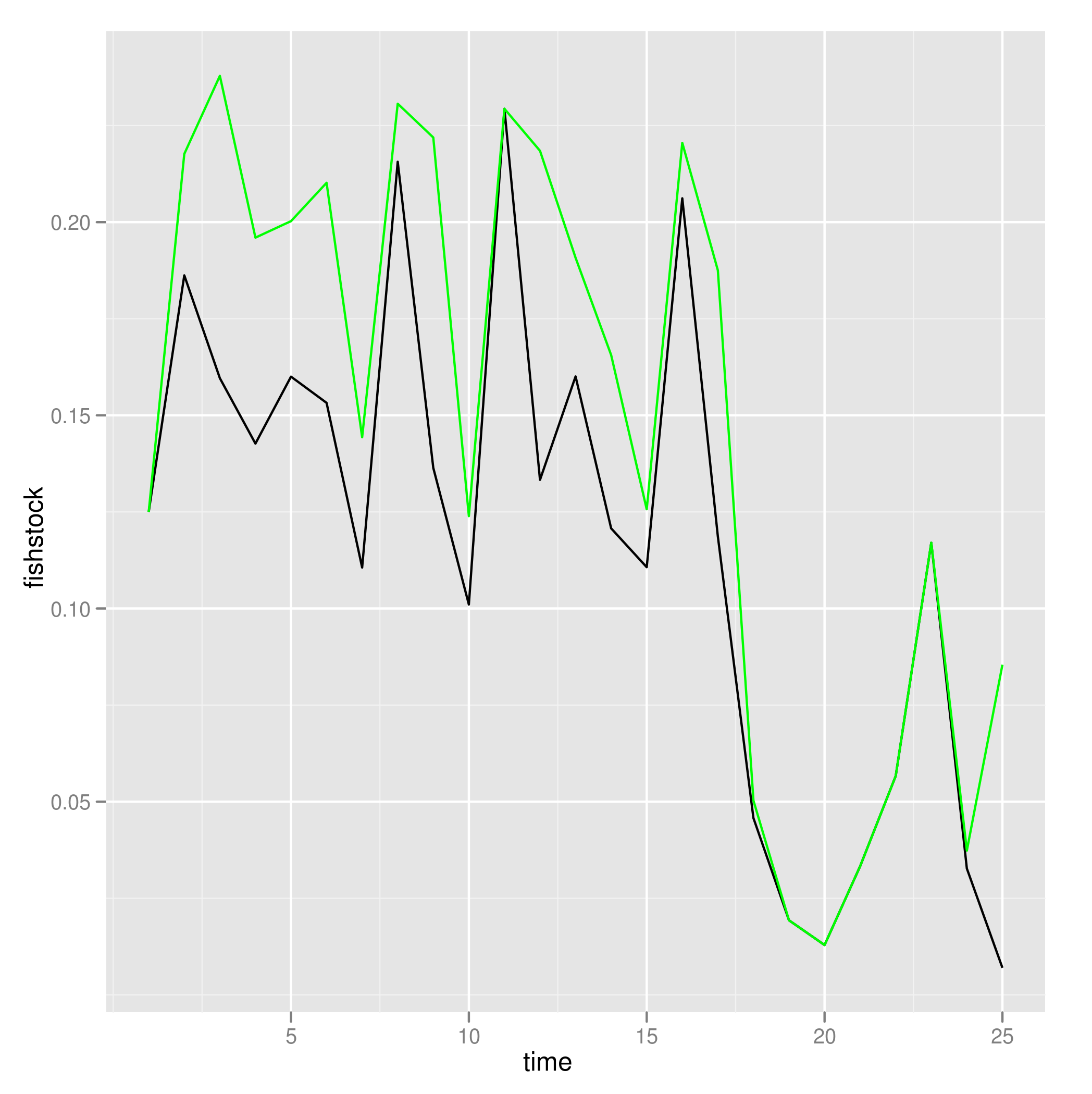
Results: Optimally harvested (black) and unharvested (green) population dynamics, for a stochastic realization.

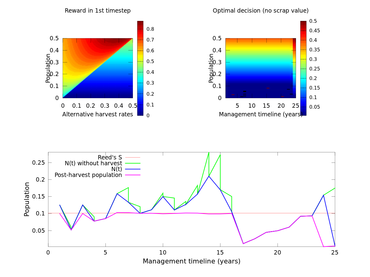
From the original Matlab example from michael (run in Octave):

- Optimal Escapement Levels in Stochastic And Deterministic Harvesting Models, William J Reed, (1979) Journal of Environmental Economics And Management, 6 10.1016/0095-0696(79)90014-7