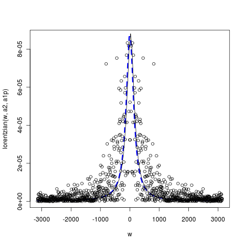
Matching the warning signal to different SDE models couldn’t retain the simplicity and generality needed, so I intend to work on the transformed data instead. Taking the power spectrum of the data, we have a new curve fitting problem:

(Code). This can be turned into a linear curve fitting problem by taking the log of the inverse Fourrier transform, then the slope is our stability parameter. Can we do this estimation by likelihood instead of least-squares? What is the error model of scatter around the Lorentzian anyway? Does this loose the temporal information of a changing rate for that parameter?
Today’s goals:
Get the inverse fft matching the theory
Compute likelihoods on the transformed data?
Compare between stationary and non-stationary models
The big challenge: how do I define a likelihood function on the transformed data? Is this even possible??
Victory! (or maybe half victory)
So after some discussion with my brother, Alistair Boettiger: yes – it is possible to fit by likelihood: Imagine transforming the entire distribution of outcomes (ensemble) into a power spectrum. This creates a “fuzzy” power spectrum, with deviations from that expected by the model. A couple useful observations let us determine that distribution:
The mean of that distribution (fuzzy Lorentzian) is the expected power spectrum of the model; so given a candidate model we can easily subtract this out.
The errors are normally distributed. This follows because (a) the distribution of the original model was normal (exactly true for our linear SDEs / Fokker-Planck models, otherwise by linear noise approximation they are close to Gaussian); (b) the Fourier transform is linear; and (c) the Fourier transform of the Gaussian is Gaussian.
This is otherwise known as great news! The exact form I probably cannot write from parameters of the model, but will allow that error to be an extra parameter – giving us the two Lorentzian shape parameters (height and width, will fix position around zero as we’re not interested in regular oscillations) and the error term. From this the likelihood is then easy to estimate from data as seen above.
Err… Almost.
The above graph clearly doesn’t seem to show normal scatter about the curve. Also, the power spectrum takes the (norm of the) square of the FFT, so we have:
\[ \left| (f(w) + N(w))^2 \right| = \left| f(w)^2 + 2f(w)N(w) +N(w)^2 \right| \]
where \(| latex f(w)^2 |\) is the Lornetzian and $ N(w)$ the normal random variate. That is, an error that looks like
\[ \left| 2 f(w)\right| \left| N(w)\right| +N(w)^2 \]
So the error does depend on the mean, just as it appears. Note that for the complex-valued function \[ | f(x) ^2 | = |f(x)|^2 \] so $ |f(x)| $ is the square root of the Lorentzian signal, $ |f(x)|^2 $
Calling the power in the data $ P(x) $ and the variance of the normal be $ ^2$ and the unit normal $ Z$, we have:
\[ (P(w) - |f(x)|^2 - \sigma^2)/(2\sigma) = f(w) \left| Z \right| +Z^2 \]
hmm.. perhaps better to simply estimate the probability density directly from the first equation specifying the PDF(w). In any event, reduces to a nice likelihood calculation I should be able to implement in the code soon.
Next up: the rate-changing model
The remaining challenge is to understand how deviations in the model, particularly various loss of stability processes, impact this fitting, and how to frame the alternative model. Presumably it is not also Lorentzian.