Adaptive Dynamics

Created plotting functions for:

waiting time distribution by phase, (cumulative and difference),
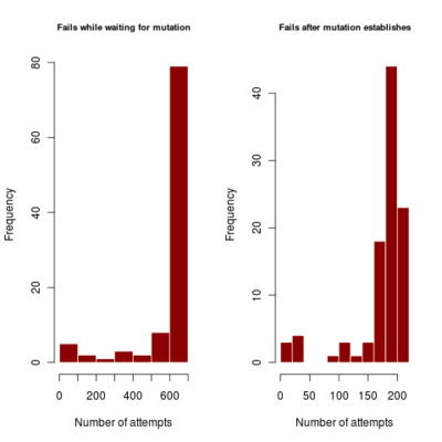
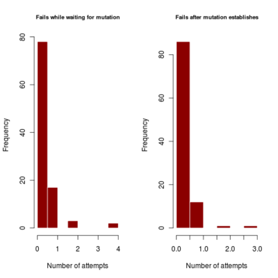
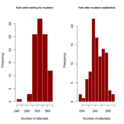
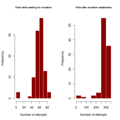
distribution of number of failures before invasion of dimophism can occur and after it has occurred (indicating if mutational rate is more limiting or mutational step size (selection gradient).
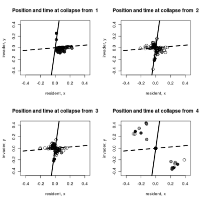
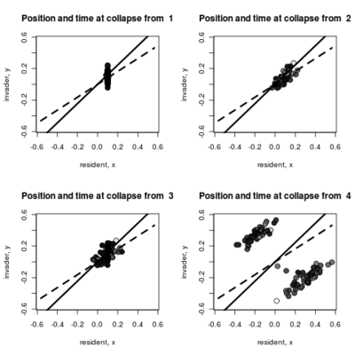
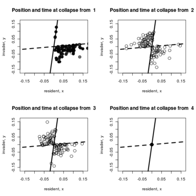
Adding to the pairwise invasibility plot the locations where dimorphism collapses, color coded by the time of collapse.

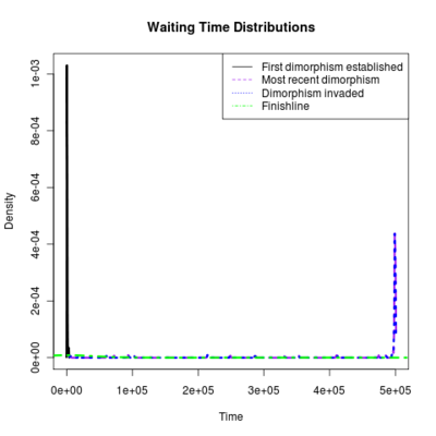
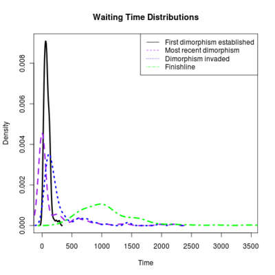
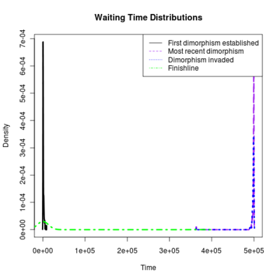
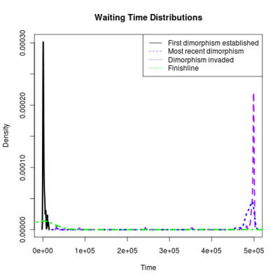
Exploring branching time distributions in different regimes by phase. Trying to figure out which parameter regimes which actually branch successfully in under 5e5 time units. Note that these aren’t timesteps, since this is Gillespie simulation; I think about birth R*Ko events occur every time unit, so an R=1, ko=500 simulations this is about 5e8, with about 2.5e4 - 2.5e5 mutations occurring in the simulation. with 100 ensembles and 4 parameter regimes this is 1e11 events. As the algorithm scales tightly on how many populations it must handle (much faster when essentially monomorphic) this isn’t directly proportional to speed, but on the 16 processor machines takes about a couple hours to run…

### Branching success by regimes tried

First set

 rep <- 100
 cpu <- 16
 all[[1]] <- ensemble_sim(rep=rep, sigma_mu = 0.05, mu = 1e-3, sigma_c2 = .8, sigma_k2 = 1, ko = 500, xo = 0.1, threshold = 30, cpu=cpu)
 all[[2]] <- ensemble_sim(rep=rep, sigma_mu = 0.05, mu = 1e-3, sigma_c2 = .1, sigma_k2 = 1, ko = 500, xo = 0.1, threshold = 30, cpu=cpu)
 all[[3]] <- ensemble_sim(rep=rep, sigma_mu = 0.05, mu = 5e-4, sigma_c2 = .8, sigma_k2 = 1, ko = 500, xo = 0.1, threshold = 30, cpu=cpu)
 all[[4]] <- ensemble_sim(rep=rep, sigma_mu = 0.05, mu = 1e-4, sigma_c2 = .3, sigma_k2 = 1, ko = 500, xo = 0.1, threshold = 30, cpu=cpu)
 
for(i in 1:4){
    png(file=paste("run2_waitingtimes_ens_", i, ".png", sep=""))
    plot_waitingtimes(all[[i]])
    dev.off()
 
    png(file=paste("run2_butterfly_ens_", i, ".png", sep=""))
    plot_butterfly(all[[i]])
    dev.off()
 
    png(file=paste("run2_failures_ens_", i, ".png", sep=""))
    plot_failures(all[[i]])
    dev.off()
}
 
> proc.time()
    user   system  elapsed 
   2.700    0.440 4685.922

corresponds to a runtime of about 78 minutes, with most simulations running to maximum time. Results in run order shown

:::::

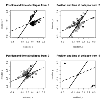
Spikes at the end of waiting times indicate simulation termination before event occurs, from runs that never branched

:::::

Trying to find parameters where more runs will finish in 5e5 max time.

all[[1]] <- ensemble_sim(rep=rep, sigma_mu = 0.05, mu = 5e-3, sigma_c2 = .8, sigma_k2 = 1, ko = 500, xo = 0.1, threshold = 30, cpu=cpu)
all[[2]] <- ensemble_sim(rep=rep, sigma_mu = 0.05, mu = 1e-3, sigma_c2 = .1, sigma_k2 = 1, ko = 500, xo = 0.1, threshold = 30, cpu=cpu)
all[[3]] <- ensemble_sim(rep=rep, sigma_mu = 0.03, mu = 5e-4, sigma_c2 = .3, sigma_k2 = 1, ko = 500, xo = 0.1, threshold = 30, cpu=cpu)
all[[4]] <- ensemble_sim(rep=rep, sigma_mu = 0.05, mu = 1e-4, sigma_c2 = .3, sigma_k2 = 1, ko = 500, xo = 0.1, threshold = 30, cpu=cpu)
 
==== Second Set ====

1 and 2 complete fine (2 is the easiest branching situation of the set clearly). 3 and 4 struggle to complete. Should try more exploratory sets before the large simulations.

(probably not worth loading second set of figures), first and second sets are reliably finishing most of time in these parameters. Quite surprising for the first since the branching point becomes very weak, but the high mutation rate makes this possible.

Updates needed for code

Simulation should have option to record full path
Recording times of coexistence

Updates needed for Notebook?

Somewhat tedious way to record results, even using the multiple uploads feature. Still, need to be able to preserve the figures and the code that creates them for each day. Wondering how the revised github wiki would fare for this…