I have recently modified the basic workflow of my lab notebook since discovering knitr. Before, I would write code files which I could track on github, push figures created by the code to flickr, and then write a notebook entry on wordpress describing what I was doing. I’d embed each figure I wanted into the entry, and each figure got an automatic link to github for the script that created it (which usually worked, though it didn’t say where in the script the command came from, and it required manually specifying the script name).
Because knitr allows me to write a single file containing code and formatted text, and will automatically display the code and embed the images, I can avoid that more convoluted workflow and just write.
 ](https://github.com/cboettig/pdg_control/blob/master/inst/examples)
What makes this so excellent is that knitr allows me to write in markdown, and github automatically displays nicely formatted markdown instead of raw script when you visit the page. So whereas before I would keep a bunch of working R scripts in projectname/demo I now keep a bunch of markdown scripts in inst/examples, ((since I’m using the R package for projects and demo/ doesn’t want non-R scripts)).
The great thing about this is that I can just click on each script and see nicely rendered text, links, code, and figures right on github.
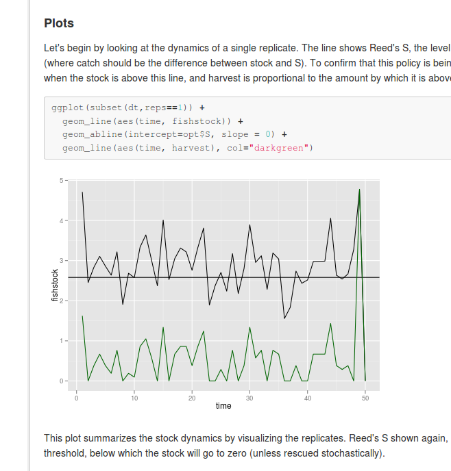 ](https://github.com/cboettig/pdg_control/blob/master/inst/examples/Reed.md)
While I can push this same markdown script to wordpress and have it be rendered in my notebook, I think maintaining these examples on github is preferable. Note that every script-name appears twice, once with and once without the _knit_ extension. The _knit_ extension indicates the file I ran to create the output (the code is in html comments so you can only see them in raw form). Because all the code is displayed in the output file (unless I call knitr options to surpress this), there’s really no need to view the _knit_ file to reproduce the example, everything is in one place in the output .md file.
These files benefit from the github managed version history, just clicking the history button gives a list of all the former versions, with code and results right there.
While I could update a post in the notebook in the same way, the version control of this wordpress notebook is more crude, and more importantly, the blog-format is designed for a linear flow, whereas in a given day I might update each of these example scripts. This seems like a much more natural workflow then having consecutive entries in the notebook with updated versions of the analysis the day before, and more natural than going back and changing a previous notebook entry.
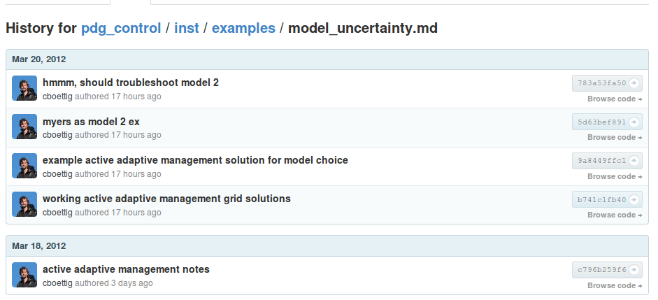 ](https://github.com/cboettig/pdg_control/commits/master/inst/examples/model_uncertainty.md)
Github can also gives nice snapshot of what’s changed, along with the commit notes for each project, for each day. Now that I can display figures and formatted text on github, as well as code, what role does the Wordpress notebook play? I think this wordpress notebook can resume is proper role as a lab notebook, containing reflections and synthesis on what I’ve done, rather than the more comprehensive copies of each analysis and each figure. Because it’s the internet, I can link to each of the analyses of that day using version-stable links from github, or links that always give the most recent version. This requires additional effort, but it’s a reflection I should be doing anyway. We’ll see how it goes. Meanwhile, welcome to the open lab notebook v2.0.
A few more details
Longer code & R functions
When I write code longer than a few lines, I try to make it a function, or collection of functions, and include basic Roxygen-style documentation with it so I don’t have to read the code to remember how to use it. These functions naturally live in the R/ directory of the project. The project’s R package can be installed, and all these functions are then available. Each of my example scripts calls functions belonging to the package, but those functions change less regularly. To fully reproduce the example, it would be necessary to grab a copy of the R package from the same commit-version as the script. In practice, most of the time any version of the package R functions could be used.
Github wiki
Github has wiki pages which I could use instead of putting my entries in inst/example, since both render markdown (the wiki will additionally render mathjax math, all be it as a png). However, the wiki is aimed at online editing, and exists as a separate repository, so just keeping the markdown files in the project directory is simpler.
Images
Github doesn’t actually host the images. In fact, my images are still being pushed to flickr, and you can see them there. Knitr is handling this automatically as the figures are created, keeping track of the links so they can be included in the output markdown. Knitr can do this with imgur out of the box, and I’ve also written a wrapper to let it push the images to a wordpress site. Doesn’t really matter where they are stored, they can always be viewed on Github.
Heavy computing
I’ve found that the knitted markdown examples make the most sense for fast-running examples. Despite excellent caching support, I’ve found it best to run really long-running examples as external R scripts, and then save and import this data. Such scripts are often being run on a cluster that can’t push images to the internet anyway.
Power of openness?
It occurs to me that this system would be harder but not impossible, in a closed environment. I could upload the figures to flickr with private status. The links are hashes, so cannot be guessed. If the output were then hosted on a secure site (running a markdown renderer, such as Jekyll), instead of github, these links would still work to display the images. Then one could give selected access to those pages. But the open solution works out of the box.