Implements a numerical version of the SDP described in (Sethi et. al. 2005).

## Clear the workspace and load package dependencies: 
rm(list=ls())   
require(pdgControl)
require(reshape2)
require(ggplot2)
require(data.table)

We consider a Beverton Holt state equation governing population dynamics, \(f(x,h) = \frac{A x}{1 + B x}\)

f <- BevHolt

With parameters A = 1.5 and B = 0.05.

pars <- c(1.5, 0.05)
K <- (pars[1] - 1)/pars[2]

Note that the positive stationary root of the model is given by \( \), or carring capacity K = 10.
We consider a profits from fishing to be a function of harvest h and stock size x, \( (x,h) = h - ( c_0 + c_1 ) \), conditioned on \( h > x \) and \(x > 0 \),

price <- 1
c0 <- 0.01
c1 <- 0
profit <- profit_harvest(price=price, c0 = c0, c1=c1)

with price 1, c0 0.01 and c1 0.

xmin <- 0
xmax <- 1.5 * K
grid_n <- 100

We seek a harvest policy which maximizes the discounted profit from the fishery using a stochastic dynamic programming approach over a discrete grid of stock sizes from 0 to 15 on a grid of 100 points, and over an identical discrete grid of possible harvest values.

x_grid <- seq(xmin, xmax, length = grid_n)  
h_grid <- x_grid

delta <- 0.05
xT <- 0
OptTime <- 25

We will determine the optimal solution over a 25 time step window with boundary condition for stock at 0 and discounting rate of 0.05. Different scenarios introduce different assumptions about the sources of noise. Unlike (Sethi et. al. 2005), we use log normal insead of uniform noise, which requires Monte Carlo integration to estimate the transition matrix. Note that we also have a Beverton-Holt recruitment function instead of the logistic map, and differ in the precise choice of parameters for the state equation, noise, discounting, profit function, etc.

Scenarios

Large Measurement error

sigma_g <- 0.01    # Noise in population growth
sigma_m <- 0.25     # noise in stock assessment measurement
sigma_i <- 0.01     # noise in implementation of the quota
z_g <- function() rlnorm(1,  0, sigma_g) # mean 1
z_m <- function() rlnorm(1,  0, sigma_m) # mean 1
z_i <- function() rlnorm(1,  0, sigma_i) # mean 1

require(snowfall) 
sfInit(parallel=TRUE, cpu=16)

R Version:  R version 2.14.1 (2011-12-22)

SDP_Mat <- SDP_by_simulation(f, pars, x_grid, h_grid, z_g, z_m, z_i, reps=19999)

Library ggplot2 loaded.

measure <- find_dp_optim(SDP_Mat, x_grid, h_grid, OptTime=25, xT=0, 
                     profit, delta=0.05, reward=0)

Large growth error

sigma_g <- 0.25    # Noise in population growth
sigma_m <- 0.01     # noise in stock assessment measurement
sigma_i <- 0.01     # noise in implementation of the quota
z_g <- function() rlnorm(1,  0, sigma_g) # mean 1
z_m <- function() rlnorm(1,  0, sigma_m) # mean 1
z_i <- function() rlnorm(1,  0, sigma_i) # mean 1

SDP_Mat <- SDP_by_simulation(f, pars, x_grid, h_grid, z_g, z_m, z_i, reps=19999)

Library ggplot2 loaded.

growth <- find_dp_optim(SDP_Mat, x_grid, h_grid, OptTime=25, xT=0, 
                     profit, delta=0.05, reward=0)

Large implementation error

sigma_g <- 0.01    # Noise in population growth
sigma_m <- 0.01     # noise in stock assessment measurement
sigma_i <- 0.25     # noise in implementation of the quota
z_g <- function() rlnorm(1,  0, sigma_g) # mean 1
z_m <- function() rlnorm(1,  0, sigma_m) # mean 1
z_i <- function() rlnorm(1,  0, sigma_i) # mean 1

SDP_Mat <- SDP_by_simulation(f, pars, x_grid, h_grid, z_g, z_m, z_i, reps=19999)

Library ggplot2 loaded.

imp <- find_dp_optim(SDP_Mat, x_grid, h_grid, OptTime=25, xT=0, 
                     profit, delta=0.05, reward=0)

require(reshape2)
policy <- melt( data.frame(stock=x_grid, implementation = x_grid[imp$D[,1]], measurement = x_grid[measure$D[,1]], growth = x_grid[growth$D[,1]]), id="stock")
value <-  melt(data.frame(stock=x_grid, implementation = imp$V, measurement = measure$V, growth = growth$V), id="stock")
ggplot(policy) + geom_point(aes(stock, stock-value, color=variable)) + ylab("escapement")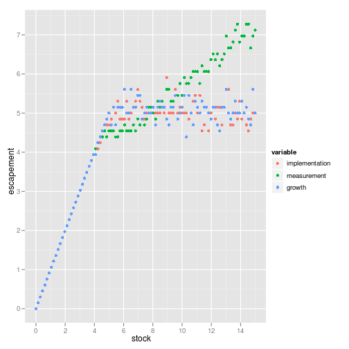

ggplot(value) + geom_point(aes(stock, value, color=variable)) + ylab("Net Present Value")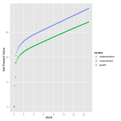

ggplot(policy) + geom_smooth(aes(stock, stock-value, color=variable))+ ylab("escapement")

ggplot(value) + geom_smooth(aes(stock, value, color=variable)) + ylab("Net Present Value")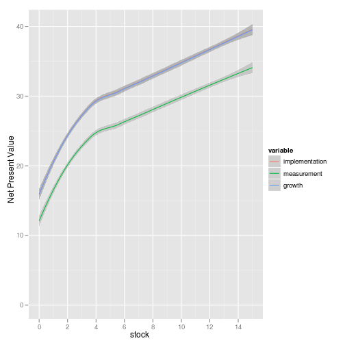

Note that growth noise gives the constant escapement solution, as expected, but large measurement noise results in raising the maximum escapement, particularly at large stock sizes. If the measured population was unusually high you might assume it was a measurement error and not increase your target harvest immediately, so this makes some intuitive sense.

author Carl Boettiger,
license: CC0
A dynamic document generated with knitr

References

Sethi G, Costello C, Fisher A, Hanemann M and Karp L (2005). “Fishery Management Under Multiple Uncertainty.” Journal of Environmental Economics And Management, 50. ISSN 00950696, doi:10.1016/j.jeem.2004.11.005