Sethi Model
- author Carl Boettiger,
- license: CC0
Implements a numerical version of the SDP described in (Sethi et. al. 2005).
Clear the workspace and load package dependencies:
Define noise parameters
sigma_g <- 0.1    # Noise in population growth
sigma_m <- 0.1     # noise in stock assessment measurement
sigma_i <- 0.1     # noise in implementation of the quota
we’ll use log normal noise functions. For Reed, only z_g will be random. Sethi et al will add the other forms of noise:
z_g <- function() rlnorm(1,  0, sigma_g) # mean 1
z_m <- function() rlnorm(1,  0, sigma_m) # mean 1
z_i <- function() rlnorm(1,  0, sigma_i) # mean 1
Chose the state equation / population dynamics function
f <- BevHoltNote that the pdg-control pacakge already has a definition for the BevHolt function, (typing the function name prints the function)
BevHoltfunction (x, h, p)
{
x <- max(0, x - h)
A <- p[1]
B <- p[2]
sapply(x, function(x) {
x <- max(0, x)
max(0, A * x/(1 + B * x))
})
}
<environment: namespace:pdgControl>That is, \( f(x,h) = \)
Of course we could pass in any custom function of stocksize x, harvest h and parameter vector p in place of BevHolt. Note that we would need to write this function explicitly so that it can take vector values of x (i.e. uses sapply), an annoying feature of R for users comming from Matlab.
We must now define parameters for the function. Note that the positive stationary root of the model is given by \( \), which we’ll store for future reference as K.
pars <- c(1.5, 0.05)
K <- (pars[1] - 1)/pars[2]
and we use a harvest-based profit function with default parameters
profit <- profit_harvest(price=1, c0 = 0.01) The profit_harvest function has the form
\[ = h - ( c_0 + c_1 ) \]
conditioned on \( h > x \) and \(x > 0 \). Note that the R code defines a function from another function using a trick known as a closure. Again we could write a custom profit function as long as it can take a vector stock size x and a scalar harvest level h. Details for provided functions can be found in the manual, i.e. ?profit_harvest.
Now we must set up the discrete grids for stock size and havest levels (which will use same resolution as for stock), in order to calculate the SDP solution. Here we set the gridsize to 100.
x_grid <- seq(0, 2 * K, length = 100)
h_grid <- x_grid
Calculate the transition matrix (with noise in growth only)
We calculate the stochastic transition matrix for the probability of going from any state \( x_t \) to any other state \( x_t+1 \) the following year, for each possible choice of harvest \( h_t \). This provides a look-up table for the dynamic programming calculations.
In the Sethi case, computing the distribution over multiple sources of noise is actually quite difficult. Simulation turns out to be more efficient than numerically integrating over each distribution. This code parallelizes the operation over four cores, but can be scaled to an arbitrary cluster.
require(snowfall)
sfInit(parallel=TRUE, cpu=4)
SDP_Mat <- SDP_by_simulation(f, pars, x_grid, h_grid, z_g, z_m, z_i, reps=999)
Library ggplot2 loaded.Note that SDP_Mat is specified from the calculation above, as are our grids and our profit function. OptTime is the stopping time. xT specifies a boundary condition at the stopping time. A reward for meeting this boundary must be specified for it to make any difference. delta indicates the economic discount rate. Again, details are in the function documentation.
Find the optimum by dynamic programming
Bellman’s algorithm to compute the optimal solution for all possible trajectories.
opt <- find_dp_optim(SDP_Mat, x_grid, h_grid, OptTime=25, xT=0,
                     profit, delta=0.05, reward=0)
Simulate
Now we’ll simulate 100 replicates of this stochastic process under the optimal harvest policy determined above.
sims <- lapply(1:100, function(i){
  ForwardSimulate(f, pars, x_grid, h_grid, x0=K, opt$D, z_g, z_m, z_i)
})
The forward simulation algorithm needs an initial condition x0 which we set equal to the carrying capacity, as well as our population dynamics f, parameters pars, grids, and noise coefficients. Recall in the Reed case only z_g, growth, is stochastic, while in the Sethi example we now have three forms of stochasticity – growth, measurement, and implementation.
Summarize and plot the results
R makes it easy to work with this big replicate data set. We make data tidy (melt), fast (data.tables), and nicely labeled.
dat <- melt(sims, id=names(sims[[1]]))
dt <- data.table(dat)
setnames(dt, "L1", "reps") # names are nice
Plots
Let’s begin by looking at the dynamics of a single replicate. The line shows Reed’s S, the level above which the stock should be harvested (where catch should be the difference between stock and S). To confirm that this policy is being followed, note that harvesting only occurs when the stock is above this line, and harvest is proportional to the amount by which it is above. Change the replicate reps== to see the results from a different replicate.
ggplot(subset(dt,reps==1)) +
  geom_line(aes(time, fishstock)) +
  geom_abline(intercept=opt$S, slope = 0) +
geom_line(aes(time, harvest), col="darkgreen") 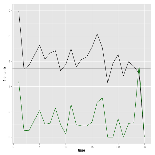
This plot summarizes the stock dynamics by visualizing the replicates. Reed’s S shown again.
p1 <- ggplot(dt) + geom_abline(intercept=opt$S, slope = 0)
p1 + geom_line(aes(time, fishstock, group = reps), alpha = 0.2)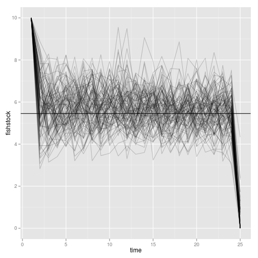
We can also look at the harvest dynamics:
p1 + geom_line(aes(time, harvest, group = reps), alpha = 0.1, col="darkgreen")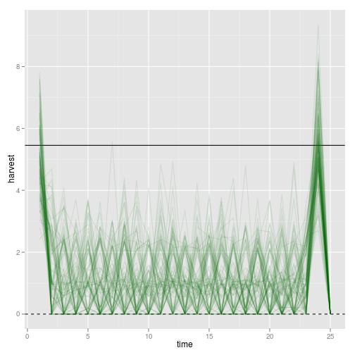
This strategy is supposed to be a constant-escapement strategy. We can visualize the escapement:
p1 + geom_line(aes(time, escapement, group = reps), alpha = 0.1, col="darkgrey")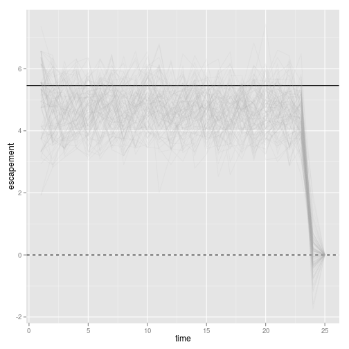
Visualizing the optimal policy
Note that when the boundary is sufficiently far away, i.e. for the first couple timesteps, the optimal policy is stationary. The optimal policy is shown here over time, where the color indicates the harvest recommended for each possible stock value at that time (shown on the vertical axis). Observe that the solution does not correspond to a simple Reed-style rule.
policy <- melt(opt$D)
policy_zoom <- subset(policy, x_grid[Var1] < max(dt$fishstock) )
p5 <- ggplot(policy_zoom) +
  geom_point(aes(Var2, (x_grid[Var1]), col=h_grid[value])) +
  labs(x = "time", y = "fishstock") +
  scale_colour_gradientn(colours = rainbow(4)) +
  geom_abline(intercept=opt$S, slope = 0)
p5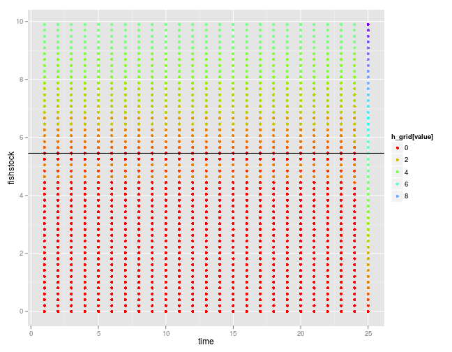
The harvest intensity is limited by the stock size.
p6 <- ggplot(policy_zoom) +
  geom_point(aes(Var2, (x_grid[Var1]), col=x_grid[Var1] - h_grid[value])) +
  labs(x = "time", y = "fishstock") +
  scale_colour_gradientn(colours = rainbow(4)) +
  geom_abline(intercept=opt$S, slope = 0)
p6 + geom_line(aes(time, fishstock, group = reps), alpha = 0.1, data=dt)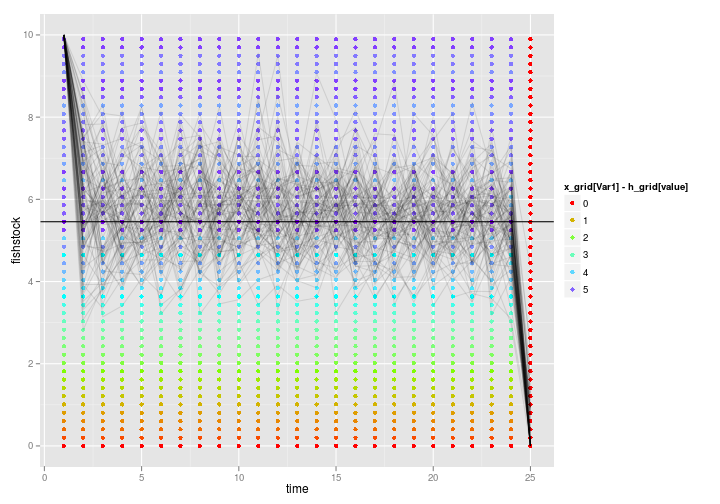
References
Sethi G, Costello C, Fisher A, Hanemann M and Karp L (2005). “Fishery management under multiple uncertainty.” Journal of Environmental Economics and Management, 50. ISSN 00950696, https://dx.doi.org/10.1016/j.jeem.2004.11.005