Summarizing efforts from last few days setting up and running some stochastic dynamic programming optimization problems. As we are focusing on discrete time at the moment, these problems are solved by Bellman’s equation (don’t need Hamilton-Jacobi-Bellman formulation).
Problem Statement
Choose the harvest level to optimize the profit \[ \max_h \sum_{t=0}^T \beta^t \pi(x,h,t) \]
Subject to the boundary conditions \(X(0) = X_0, X(T) = X_T\) and the state equation: \[ X(t+1) = Z(t) f(X(t)) \]
Where \(Z(t)\) is a normal random variable with mean unity and standard deviation \(\sigma\).
Stochastic Transition Matrices
The problem is discrete in time, but we must still discritize the state and control variables. We define the state (population abundance) to assume only the values on a grid of size \(N\). In general the control variable could be defined on a separate grid (for instance, if we used effort-control) but as harvest is in the same units as the state variable (number of fish), we can use the same grid.
The transition matrix $ maps all states \(x_i\) to all other states \(x_j\) by their transition probabilities through the state equation: \[ P(x_j | x_i ) = \mathcal{N} \text{lognormal}\left( \frac{x_j}{f(x_i-h)}, \sigma \right) \]
Where \(\mathcal{N}\) is just a normalization, \(\mathcal{N} = \sum_j P(x_j | x_i) = 1\). Note that the state equation is computed on the post-havest population \(x_i - h\), and hence a different matrix is produced for each possible value of \(h\) (for the moment we ignore the possibility that this function may vary explicitly with time as well, which would further increase the memory needed).
The stochastic dynamic programming solution just implements Bellman’s equation: \[ V_{t} = \max_h \left( \mathbf{T}_h V_{t+1} + \pi(x_t, h_t) e^{-\delta (T-t)} \right) \]
We begin with some final value \(V_T\) a vector of the “scrap” value of each possible end state. For instance, we can offer a fixed profit for all states above \(X_T\), and nothing otherwise. We then just iterate backwards, at each time-point trying all possible h values in the grid (from our set of transition matrices \(\mathbf{T}_h\) ) and selecting the best harvest level for each possible system state \(x_t\). Note this differs a bit from the way the boundary conditions are enforced in the deterministic continuous time case, and the exact value we put here may make a difference in different stochastic realizations.
Implementation
This is implemented in matlab code in the functions: determine_SPD_matrix.m, find_dp_optim.m, using population dynamics and profit model specified in Reed_SDP.m. We can then simulate under the state equation, and apply the optimal solution (ForwardSimulate.m) and plot the results (draw_plots.m).
This is also implemented in R, with the optimization methods specified in stochastic_dynamic_programming.R, run for selected profit function and population dynamics in Reed.R. We can explore a few examples using the R code.((recall that figures link to code snapshot, click through to see parameter values used in the script, etc))
Example exploration
Let’s assume a cost function of the from:
\[ \pi(h) = p h - c/h \]
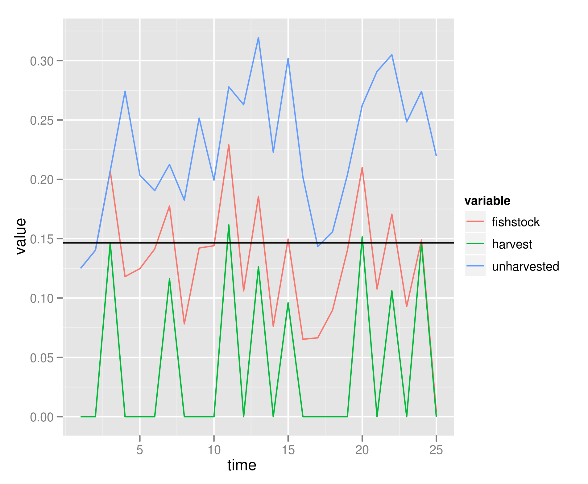
Which assumes a fixed price $ p $ and fishing costs following the Schaeffer production function. Let’s start with our allee effect model \[ f(x_t) = x_t e^{ \alpha \left(1-\frac{x}{K}\right) \left( \frac{x-C}{K} \right) } \] First, with low noise, it is easy to make sure the dynamics are behaving properly:
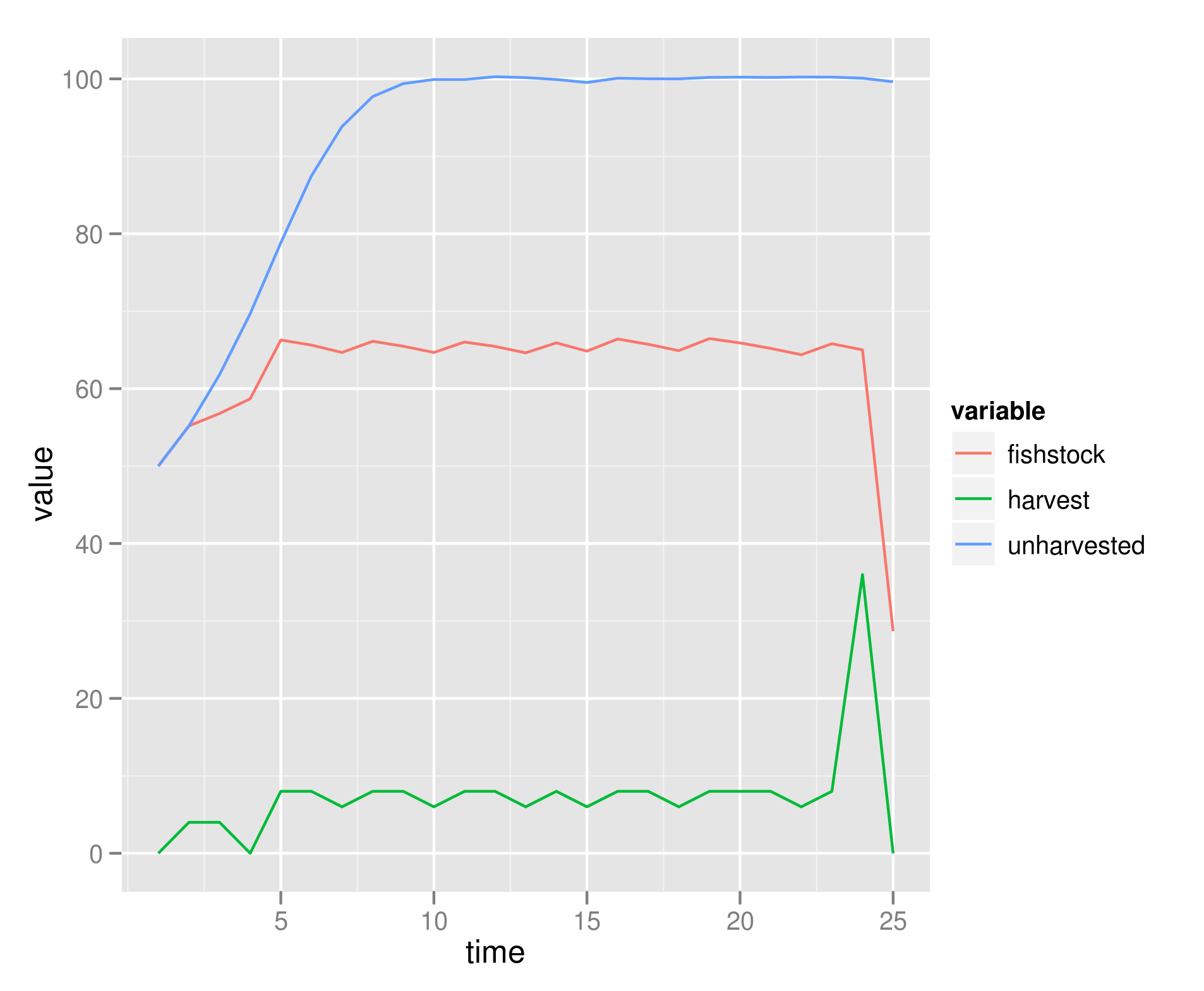
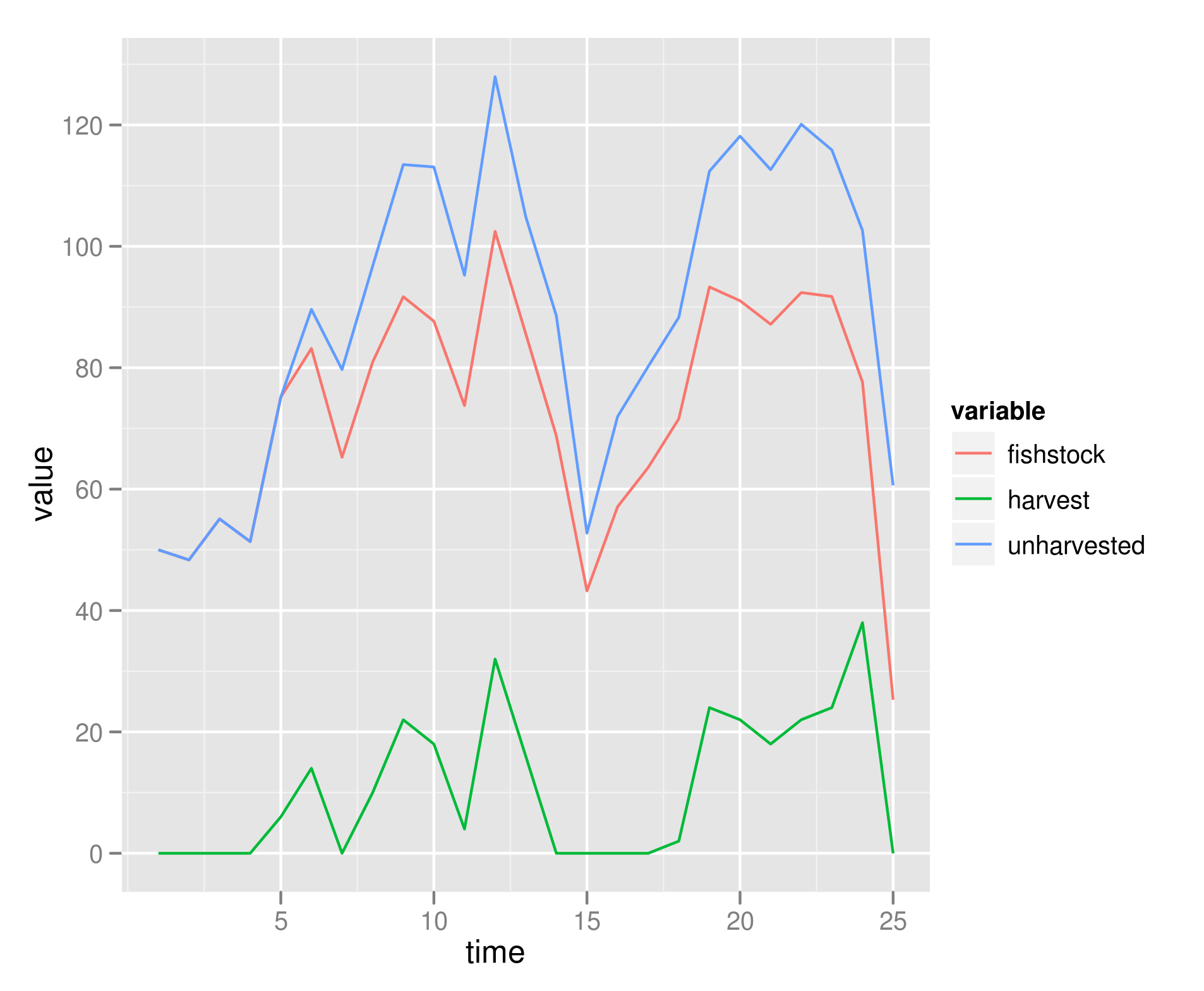
Note that the population finishes near 30, the set boundary condition. This varies with larger noise:
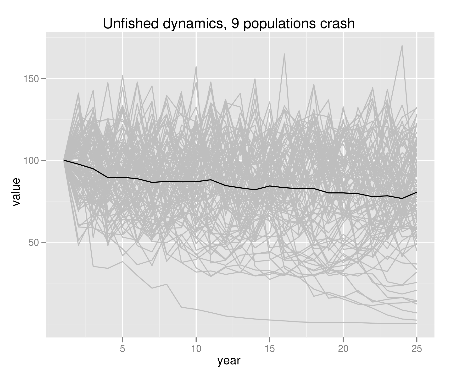
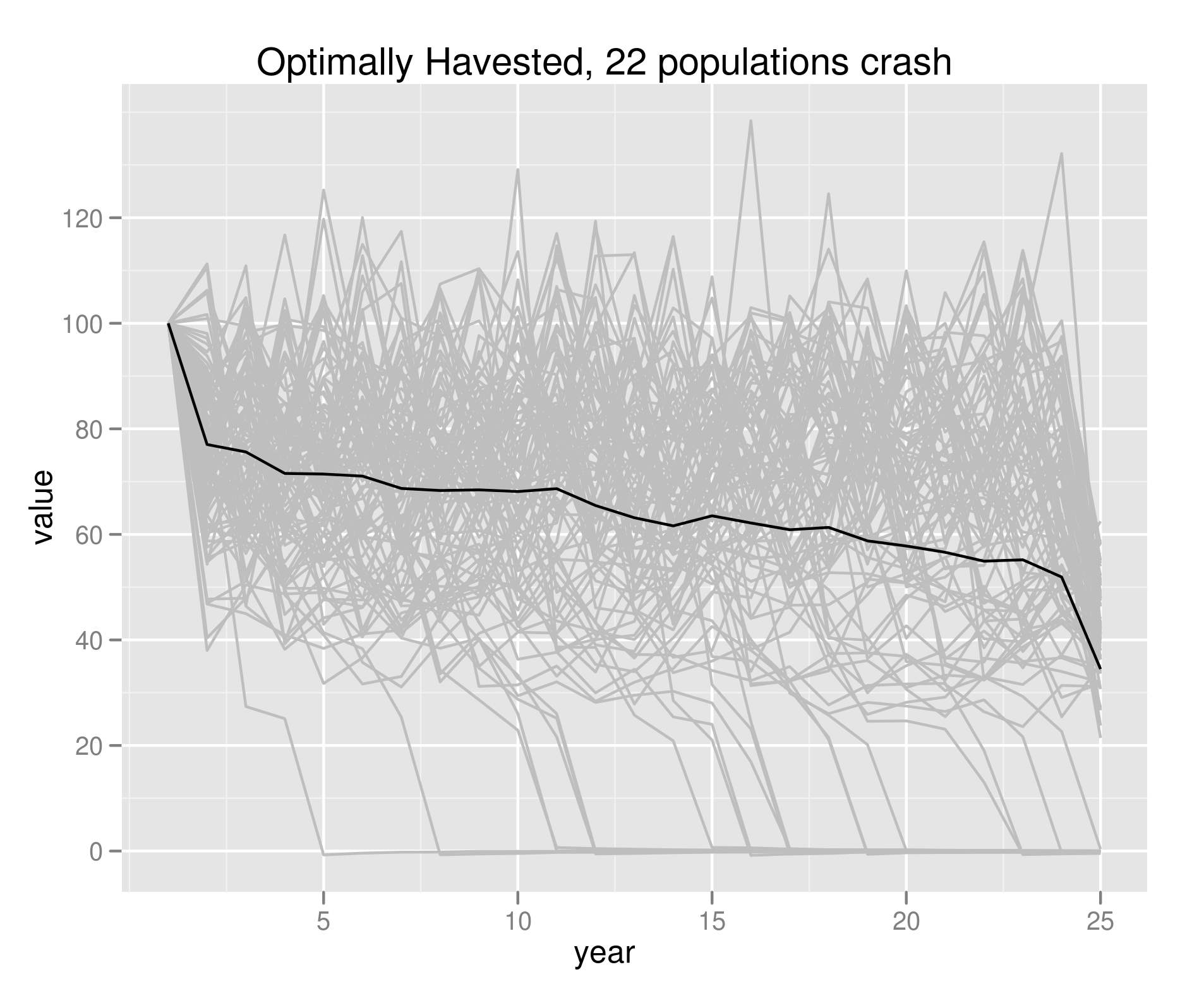
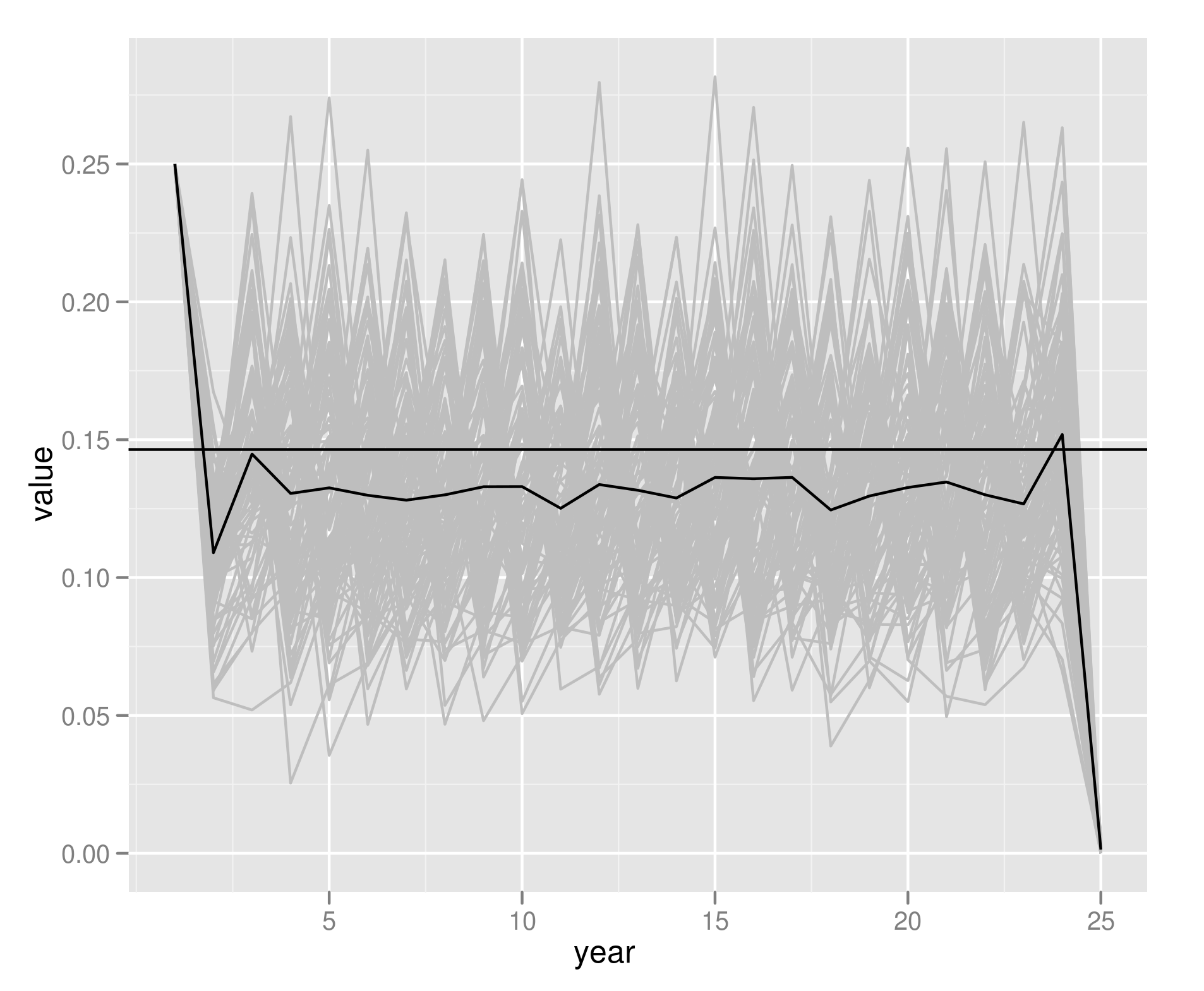
We can run a suite of replicates, and compare optimally harvested and unharvested outcomes.
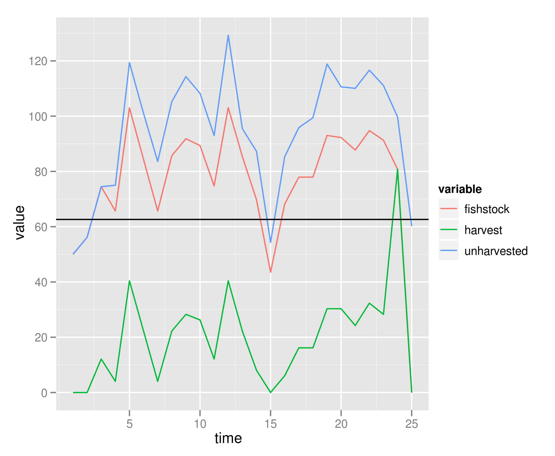
Can compare this to Reed’s optimal escapement. Let’s start with a simpler set of population dynamics using the basic Beverton-Holt model, then we harvest only whenever the population exceeds Reed’s optimal escapement threshold, $S $, and we harvest the population at a rate that should return it to $ S $ if next year’s growth were the equal to the expected growth:
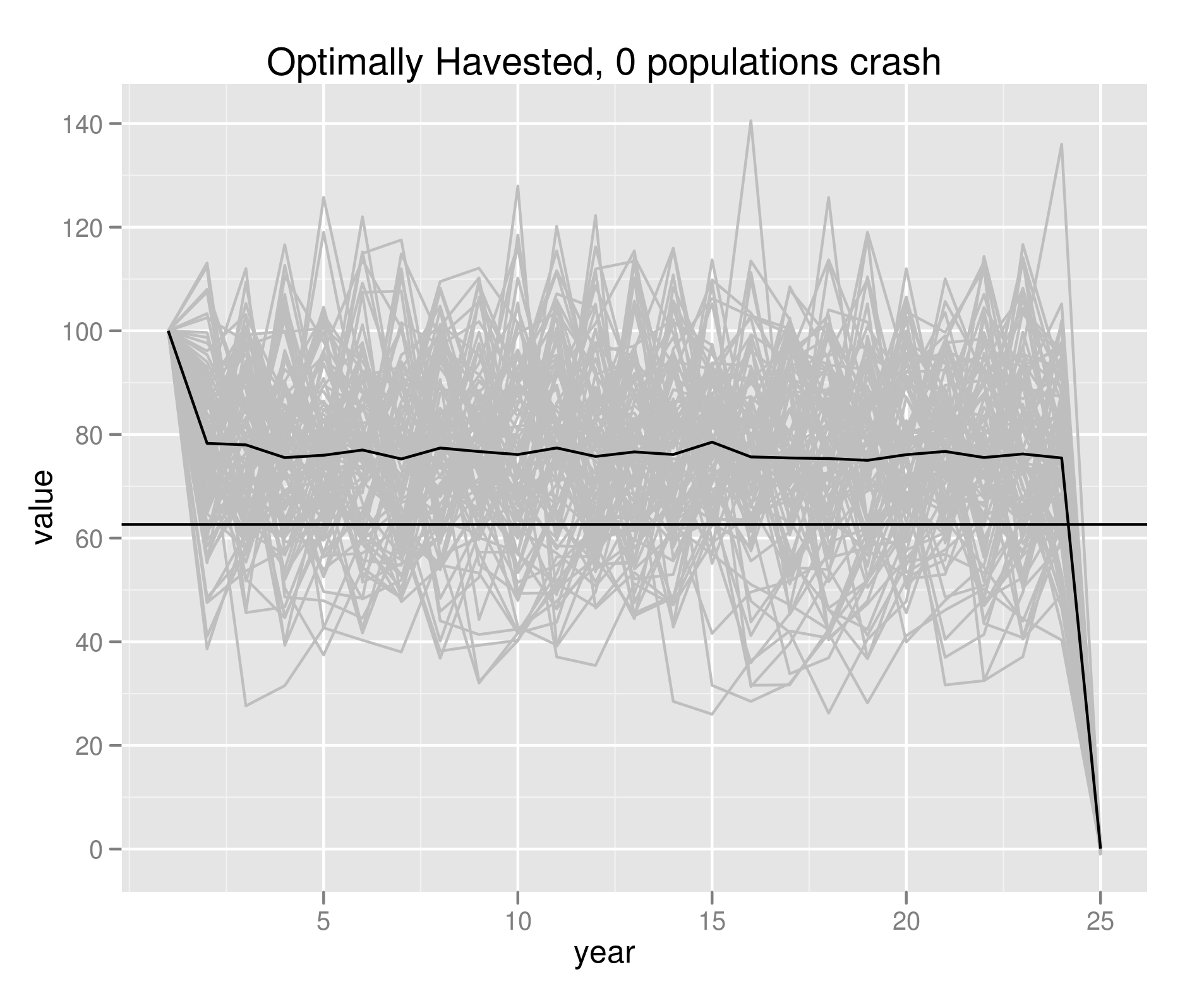
Note that this means that the average population will be below the optimal escapement, because of the curvature of the growth rate function and Jensen’s inequality:
Compare to the case of our Allee-Ricker function, even when the allee threshold is 0, the curvature is the other way, and this rule results in under-havesting more than over-harvesting the optimal escapement:
Kinda suggests that there should be a curvature-correction to Reed’s derivation, presumably that’s been done somewhere?