Discrete-time state equation
Discrete-time solution appears to be all about dynamic programming
and a chance for me to remember that I’m out of practice writing recursive functions. It’s just that in thinking about the problem, you start from the end, with the trivial subcase, and keep adding the layers. But the recursive function kinda starts at the beginning, and that trivial case is the exit condition. R doesn’t seem very efficient with these recursive functions, so this might become a C sub-routine eventually.
Problem setup
We consider some discrete-time state equation for (fish stock, \(x\)) under some control parameter (harvest, \(h\)):
\[ x_{t+1} = f(x_t, h) \]
We again have utility function, \(\pi(h)\) for diminishing returns on fish harvest. Discrete time means we maximize over the discrete discounting rate \(\beta\) and sum over intervals:
\[ \max_{h_t} \sum_{t=0}^T \beta^t \pi(h) \]
subject to the state equation above and some boundary conditions \(x_0 = X_0, \qquad x_T = X_T\). First-order conditions are:
\[ U'(h_t) = \beta U'(h_{t+1}) F'(x_{t+1} ) \forall t \] and solution will use a dynamic programming approach of the following recursion
\[ V(x_t) = \max_h \left( U(h) + \beta V(x_{t+1} ) \right) \]
Which substituting in the state equation gives us:
\[ V(x_t) = \max_h \left( U(h) + \beta V( F(x_t)) \right) \] Let’s assume a discrete Ricker-style model: \[ x_{t+1} = f(x,h) = x \exp \left( \alpha \left(1-\frac{x}{K}\right) \left( \frac{x-C}{K} \right) \right) - h x \]
The Ricker-style formulation in analogy to our continuous time problem, Alan suggests we actually consider the case by Myers et al., (Myers et. al. 1995)
\[N_{t+1} = \frac{r N_t^{\alpha}}{1+\frac{N_t^{\alpha}}{K} } \]
Trivial case of no cost at boundary, harvests everything.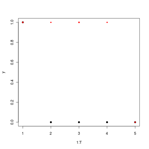
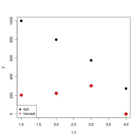
A simpler case
Fish remaining are whatever wasn’t harvested yet: \[ x_{t+1} = x_t - h_t \]
Cost/profit of harvesting: Profit \(p(t)\) per fish (possibly varies with year), but cost gets harder \(c h^2\), \(c << p(t)\), \[ U(h) = p h - c h^2 \]
The algorithm can be specified by recursion,
phi <- function(x) 300

J <- function(t,x){
  if(t < T)
    out <- U(t,x, h_star(t,x)) + beta*J(t+1, f(t,x, h_star(t,x)))
  else
    out <- phi(x)
  out
}

h_star <- function(t,x){
    func <- function(h) U(t, x, h) + beta*J(t+1, f(t,x,h))
#    optimize(f=func, interval=c(0,1))[[1]]
    h <- seq(0,1000,length=500)
    cost <- sapply(h, func)
    i <- which.max(cost)
    h[i]
}
See full code.
but this is terribly inefficient.
A simple dynamic programming reference here.
Stochastic Optimal Control
Looks like this needs a dynamic programming approach. A useful reference.
Higher-dimensional state equations
Can these lead to oscillating solutions in as the number of state equations increases? Depends on nature of constraints? Inequalities?
Steps check list
Simple boundary-value problem solution by collocation. Example.
Chebychev polynomial collocation
Harvest vs fishing effort as control variable.
Solution under inequality bounds
Discrete-time state equations
Stochastic Control
Parrotfish 3 dimensional system, Horan 2 dimensional system. See (Mumby et. al. 2007), (Blackwood et. al. 2010) (Horan et. al. 2011)
Uncertainty
References
Myers R, Barrowman N, Hutchings J and Rosenberg A (1995). “Population Dynamics of Exploited Fish Stocks at Low Population Levels.” Science, 269. ISSN 0036-8075, https://dx.doi.org/10.1126/science.269.5227.1106.
Mumby P, Hastings A and Edwards H (2007). “Thresholds And The Resilience of Caribbean Coral Reefs.” Nature, 450. ISSN 0028-0836, https://dx.doi.org/10.1038/nature06252.
Blackwood J, Hastings A and Mumby P (2010). “The Effect of Fishing on Hysteresis in Caribbean Coral Reefs.” Theoretical Ecology, 5. ISSN 1874-1738, https://dx.doi.org/10.1007/s12080-010-0102-0.
Horan R, Fenichel E, Drury K and Lodge D (2011). “Managing Ecological Thresholds in Coupled Environmental-Human Systems.” Proceedings of The National Academy of Sciences, 108. ISSN 0027-8424, https://dx.doi.org/10.1073/pnas.1005431108.