Discussed \(\text{MC}^3\), the Metropolis coupled Markov Chain Monte Carlo, in Monday’s algorithms group meeting, just getting around to posting code. The MrBayes paper is a good reference for this (Altekar et. al. 2004). Ourpractice example needed some debugging. I re-wrote a general purpose mcmcmc function in R to illustrate the algorithm, below. Recall that it modifies our original MCMC in two ways. The normal proposal step gets weighted by temperature, allowing heated chains to step downhill more often. We draw a uniform (0,1) random number and accept the move R is larger than it, where:
\[ R = \min\left[ 1, \left( \frac{f(X|\theta^{\prime})}{f(X|\theta)} \times \frac{f(\theta^{\prime})}{f(\theta)} \right)^{\beta_i} \times \frac{q(\theta)}{q(\theta^{\prime})} \right] \]
where
\[ \beta_i = \frac{1}{1+\Delta T \times (i-1)} \]
for priors $ f() $, likelihood $ f(X|) $, proposed parameters $ ^{} $, and proposal density $ q() $
In this mode chains evolve along independently. We occasionally propose a swap between chains, where the Hastings ratio takes on the specific form:
\[R = \min \left[1, \left( \frac{f(\theta_k|X)}{f(\theta_j|X)} \right)^{\beta_j} \left( \frac{f(\theta_j|X)}{f(\theta_k|X)}\right)^{\beta_k} \right]\]
Note that for the posterior $ f(| X) $ we use $ f(X|) f() $, just as in the single chain case, which is true modulo the normalization $ f(X) $.
[gist id=981399]
Note this code doesn’t run anything, we have to specify temperature ratios $ _i $, the likelihood function, and the prior, and then it can give us back chains. Here’s a trivial example based on our Gaussian process:
## Observed Data
X <- rnorm(20, 2, 5)

loglik <- function(pars){
  ## The likelihood function
  sum( dnorm(X, mean=pars[1], sd=pars[2], log=TRUE) )
}
prior <- function(pars){
1/pars[2]^2
#  dnorm(pars[1], 0, 1000, log=TRUE)+
 # dnorm(pars[2], 0, 1000, log=TRUE)
}

# chains can have different or matching starting conditions, will mix anyway
pars <- list(c(1,2), c(1,2))

chains <- mcmcmc_fn(pars, loglik, prior, MaxTime=1e3, indep=100, stepsizes=.02)
Works rather well: 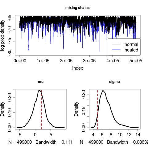
With different prior:
prior <- function(pars){
  dnorm(pars[1], 0, 1000, log=TRUE) + dexp(pars[2], 10, log=TRUE)
}
The run converges on an erroneous sigma value:
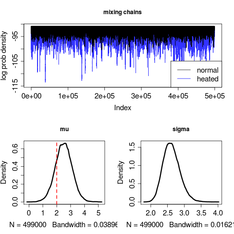
Longer runs don’t seem to fix this, but increasing the number of sample points in the data (from 20 to say, to 200) does.
Plotting code:
layout(t(matrix(c(1,1,2,3), nrow=2)))
par(cex.lab=1.5, cex.axis=1.5)
plot(chains[[2]][-burnin, 1], type='l', col=rgb(0,0,1,.8),
 main="mixing chains", ylab="log prob density")
lines(chains[[1]][-burnin, 1], col="black")
legend("bottomright", c("normal", "heated"), col=c("black", "blue"), lty=1,cex=1.5)
plot(density((chains[[1]][-burnin, 2])), lwd=3, main="mu")
#curve(dnorm(x, 0, 1000), add=TRUE, lty=2)
abline(v=2, col="red", lwd=2, lty=2)
plot(density((chains[[1]][-burnin, 3])), lwd=3, main="sigma")
#curve(dexp(x, 10), add=TRUE, lty=2)
abline(v=5, col="red", lwd=2, lty=2)
References
- Altekar G, Dwarkadas S, Huelsenbeck J and Ronquist F (2004). “Parallel Metropolis Coupled Markov Chain Monte Carlo For Bayesian Phylogenetic Inference.” Bioinformatics, 20. ISSN 1367-4803, https://dx.doi.org/10.1093/bioinformatics/btg427.