Continuing my exploration in applying these techniques to real climate data. Applying the Kendall’s Tau based approach on real data.
Greenhouse Earth, CaCO3 data:
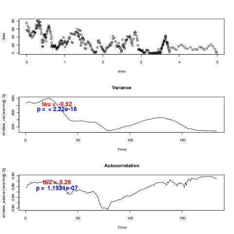
Glaciation I-IV (deuterium data)
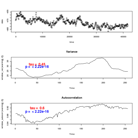
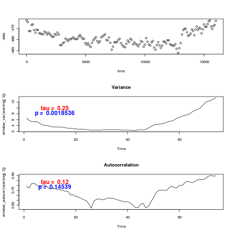
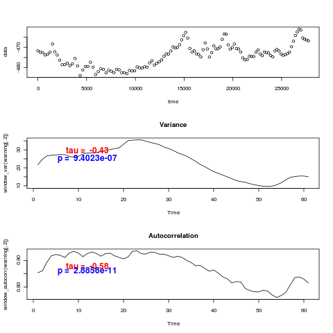
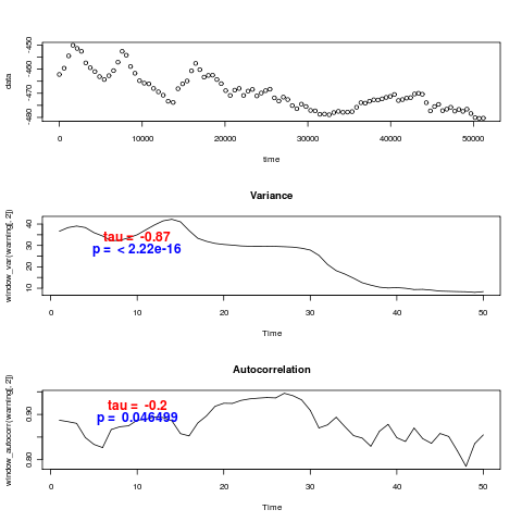
These use the unadjusted timeseries, and hence don’t reproduce the values of Kendall’s tau statistic reported in (Dakos et. al. 2008). In fact they don’t even agree on the sign – visually many of the datasets are certainly decreasing in variance. I ran the Monte-Carlo distributions for tau on models estimated from these data-sets with and without warning, for variance (left) and autocorrelation (right), in the CaCO3 data:
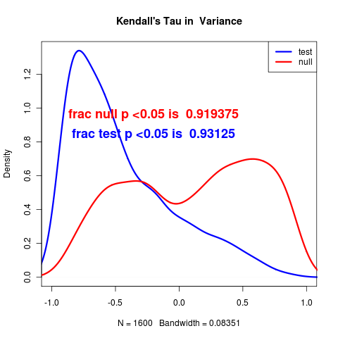
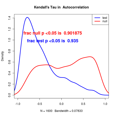
and again the models with a trend show an actual decrease in the variance and autocorrelation, (just as the real data does), as well as rather low power to distinguish. The opposite trend is observed by (Dakos et. al. 2008) after detrending and interpolating the data.
Detrending and Interpolating
We can try both interpolating and detrending the data to compare more directly (R functions make this easy. We follow the original work using ksmooth for kernel smoothing mean which is subtracted out, and approx for linear interpolation).
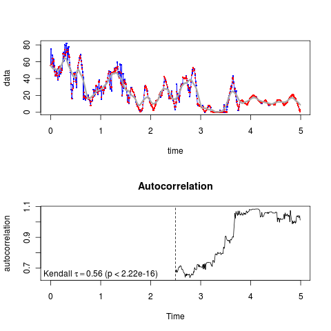
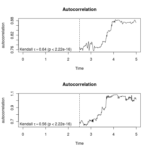
Top plot shows the raw data (blue), interpolated data (red) and trend subtracted from the data (gray). Lower curve shows the autocorrelation, AR1 coefficient over the moving window and it’s score in Kendall’s tau test.[ref] Note some effort required to produce these nicer plots. Particularly, R makes it rather unintuitive how to specify that a greek letter is equal to a variable. expression is typically used to display math/greek, but doesn’t work for including values of a variable. After wasting some time, posted to our statcompsci lsit and got the answer in about 30 seconds from Duncan: the key is the substitute command. See the code in show_stats function in the tau_dist_montecarlo.R file.[/ref]
Supplement describes the functions used by (Dakos et. al. 2008), many of which are from R (some, like linear interpolation, is done in matlab). They use autocorrelation calculated with “ar.ols”, while I have been using the acf function. I compare the differences with warning_ar.ols with warning_autocorr (acf) (right; code) The ar.ols is substantially slower to evaluate (seconds per call on this data). I also migrated to the built in cor.test(method=“kendall”) in “stats” package rather than the “Kendall” function in the extension package “Kendall” for consistency.
Now set to rerun the above results on the detrended, interpolated data…
References
- Dakos V, Scheffer M, van Nes E, Brovkin V, Petoukhov V and Held H (2008). “Slowing Down as an Early Warning Signal For Abrupt Climate Change.” Proceedings of The National Academy of Sciences, 105. ISSN 0027-8424, https://dx.doi.org/10.1073/pnas.0802430105.