Primates project now has a Github repository. Updates are embedded from here.
Experimenting with distributing code and data effectively. Pluses and minuses of three options:
- zipped file with R code and data. Requires setting working directory, harder to update. Subsequent uploads must include all the data, rather than incremental.
- Directly grab repository over github. Simple to update and access, stores only incremental changes. Requires knowledge of git
- R package: Nicely integrates data, code, and documentation. Requires installing R packages.
- Learning the R packaging system for data. You can have .R files in the data/ directory of a package. The call to the data() function runs those files from that directory, making it unnecessary to specify the path to the data and allowing the use of complicated functions, see the example from the ape package:
require(ape, quietly = TRUE, save = FALSE)
bird.orders <- read.tree("bird.orders.tre")
Primate Phylogeny —————–
Carl Boettiger 00:37, 30 April 2010 (EDT):
- Simon sent me the tree data from their paper:
- Chatterjee HJ, Ho SY, Barnes I, and Groves C. . pmid:19860891. PubMed HubMed [primates]
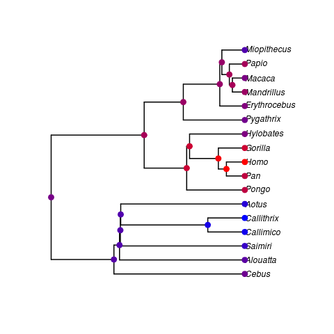
- This is the first calibrated ultrametric tree I’ve been able to couple to the primate data Daniel provided. I’ve preformed a quick ancestral state reconstruction on log brain weight (warmer colors are more massive).
### R code to create figure
library(ape)
library(geiger)
genera_set <- read.nexus("mt.genera.ucld.trees")
nuc_set <- read.nexus("nuc.ucld.trees")
genera <- genera_set[[1]]
nuc <- nuc_set[[1]]
nuc_names <- nuc$tip.label
genera_names <- genera$tip.label
traits <- read.csv("Primate_brain_comparisons.csv")

dups <- duplicated(traits[['Genus']])
trait_names <- as.character(traits$Genus[!dups])
x <- traits$log_brain.weight[!dups]
names(x) <- trait_names


compare <- treedata(nuc, x)
plot(compare$phy)
out <- ace(compare$data, compare$phy)

# a similar function but for the continuous ancestral state
plot_cts_ancestor <- function(phy, data, ancestral){
    plot(phy) # just to get treelength
    treelen <- max(axisPhylo() )
    plot(compare$phy, cex=1, x.lim=1.3*treelen, edge.width=2)
    mycol <- function(x){
    tmp = (x - min(data)) /max(x-min(data))
    rgb(blue = 1-tmp, green=0, red = tmp )
    }
    nodelabels(pch=19, col=mycol(ancestral$ace), cex=1.5  )
    tiplabels(pch=19, col=mycol(data), cex=1.5, adj=0.5) # add tip color code
    }
plot_cts_ancestor(compare$phy, compare$data, out)- This is essentially just at the proof of concept level. A couple obvious steps:
- This uses a single tree from the posterior distribution of trees, which we’ll eventually want to average over in the parameter estimation. Meanwhile should use a consensus MLE tree instead.
- Trees are resolved to genus level, so traits should be genus averages (instead of subsamples).
- Ancestral state reconstruction under the Brownian Motion model is the most preliminary treatment, will certainly be interesting to consider the various multi-peak OU models and identify potential transitions between peaks, as well as power analysis for the model fits.
- Multidimensional trait inference should also be interesting
- Possible bug? The Homo/Pan and Gorilla/Pan nodes would be expected to be in the Gorilla/Pan colour rather than the Homo colour.
Code and data on Github
New github repository for sharing code and data: sandbox
- Grab this repository using git:
git clone git://github.com/cboettig/sandbox.git- Revert to this edit’s version of code and data using git:
git checkout 77af6613db294ca068cfDownload the snapshot as an R package. More information on the downloads page of repository.
- Carl Boettiger 16:17, 5 May 2010 (EDT):
Updated git version using R package is:
git checkout b1a90ad97b90d9cbeaa7